
LEARN · CLASSICAL MACHINE LEARNING
A machine learning model predicts that an e-commerce order has a 90% probability of arriving late. Your operations team trusts that prediction, prioritizes the shipment, and spends money on an intervention.
But when you examine thousands of similar predictions, something troubling emerges: the model is correct only 60% of the time when it claims 90% confidence.
The model might still have excellent classification accuracy. Its ROC-AUC might look respectable. It might even outperform competing models on your usual validation metrics.
Yet its probabilities are dangerously misleading.
This is the problem of model calibration, one of the most important—and frequently overlooked—aspects of production machine learning.
In this tutorial, we’ll build a deliberately overconfident classifier, diagnose its behavior with reliability diagrams, and repair its probabilities using two established techniques:
-
Platt scaling: A parametric sigmoid-based calibration method.
-
Isotonic regression: A flexible, nonparametric calibration method.
We’ll use Python and scikit-learn, generate our own synthetic delivery dataset, and measure the results with Brier score, log loss, ROC-AUC, and expected calibration error.
By the end, you’ll understand why a highly accurate classifier can produce terrible probabilities, how calibration actually works, and when recalibration can make your model worse.
1. What does it mean for a model to be calibrated?
Suppose your classifier predicts the probability that an order will arrive late.
Consider three groups of predictions:
| Predicted probability | Observed late-delivery rate | Interpretation |
|---|---|---|
| 10% | 11% | Approximately calibrated |
| 50% | 49% | Approximately calibrated |
| 90% | 60% | Severely overconfident |
A perfectly calibrated model satisfies a simple condition:
Among all predictions assigned probability p, approximately p × 100% of the corresponding events should occur.
If your model assigns a 0.80 probability to 1,000 orders, approximately 800 should actually arrive late.
This does not mean every individual prediction will be correct. A 90% probability still allows the event not to occur 10% of the time.
Calibration is a property of predictions evaluated across comparable cases, not a guarantee about any particular observation.
Formal intuition
For binary classification, define:
-
Y = 1 when an order arrives late.
-
Y = 0 when an order arrives on time.
-
p̂ = the model’s predicted probability that Y = 1.
Perfect calibration means:
P(Y = 1 | p̂ = p) = p
In practical datasets, exact predicted probabilities rarely repeat. We therefore estimate calibration by grouping predictions into probability ranges.
For example, we might examine all observations with predicted probabilities between 0.85 and 0.95.
If their average predicted probability is 0.90 but their observed event frequency is 0.60, the model is overconfident in that region.
The distinction between the model’s predicted event probability and its confidence in the predicted class will matter later.
2. Accuracy, discrimination, and calibration are different
These concepts are related, but they measure fundamentally different things.
Classification accuracy
Accuracy asks:
How often does the model choose the correct class?
A model predicting 0.51 for every positive example and 0.49 for every negative example could achieve perfect classification accuracy on a particular dataset.
However, those probabilities communicate considerable uncertainty.
Discrimination
Discrimination asks:
Can the model rank positive examples above negative examples?
ROC-AUC measures ranking quality.
A classifier could assign positive examples probabilities near 0.95 and negative examples probabilities near 0.80.
Its ranking could be perfect, producing ROC-AUC = 1.0, while its probabilities remain badly calibrated.
Calibration
Calibration asks:
Do the predicted probabilities correspond to actual event frequencies?
A calibrated model can have modest discrimination.
For example, if 30% of all orders arrive late, a model that always predicts 0.30 is calibrated at that single prediction value, provided the evaluation population has the same 30% event rate.
However, it offers no discrimination between orders. Its ROC-AUC is 0.5 when both classes are present.
The important lesson is:
A model can be well calibrated but useless for ranking, or excellent at ranking but unreliable for probability-based decisions.
Ideally, production models should have both good discrimination and good calibration.
3. Reliability diagrams: the first diagnostic tool
A reliability diagram visualizes the difference between predicted probabilities and observed event frequencies.
For binary classification:
-
The horizontal axis displays average predicted positive-class probability.
-
The vertical axis displays the observed fraction of positive examples.
-
The diagonal line represents perfect calibration.
Imagine three points on a reliability diagram:
| Average predicted probability | Actual positive frequency |
|---|---|
| 0.20 | 0.21 |
| 0.50 | 0.52 |
| 0.90 | 0.60 |
The first two points lie close to the perfect-calibration diagonal.
The third lies substantially below it.
That indicates overconfidence: the model predicts the positive event more frequently than it actually occurs.
Conversely, if a group has a predicted probability of 0.60 and an observed event frequency of 0.85, the model is underconfident about the positive event.
Why binning matters
Reliability diagrams typically divide predicted probabilities into bins.
Two common strategies are:
Uniform-width binning
Divide the probability interval from 0 to 1 into equal-width segments.
For ten bins, the ranges are approximately:
-
0.0–0.1
-
0.1–0.2
-
0.2–0.3
-
…
-
0.9–1.0
This approach makes the probability ranges intuitive.
However, if most predictions fall near 0 or 1, middle bins may contain very few examples.
Quantile binning
Divide predictions into groups containing approximately equal numbers of observations.
This usually produces more stable empirical frequency estimates, although the probability ranges have unequal widths.
Neither strategy is universally superior.
For serious calibration analysis, inspect both the reliability diagram and the number of predictions contributing to each region.
A curve without sample counts can be misleading.
4. Why some model families become overconfident
Here is the surprising fact at the center of this tutorial:
Not every classifier that supports probability prediction actually learns trustworthy probabilities, and some widely used algorithms have characteristic calibration problems.
The underlying learning objective matters.
Logistic regression: often calibrated naturally
Logistic regression directly optimizes a probabilistic objective based on log loss.
Under suitable conditions—including a reasonably specified model, representative data, and appropriate regularization—it often produces well-calibrated probabilities without additional postprocessing.
This is one reason logistic regression remains a strong baseline for probability estimation.
But it is not guaranteed to be calibrated.
Misspecified relationships, excessive regularization, distribution shift, or training procedures that distort the target prevalence can all produce unreliable probabilities.
Naive Bayes: often dramatically overconfident
Naive Bayes classifiers assume features are conditionally independent given the class.
Suppose a delivery model receives ten highly correlated measurements describing route difficulty.
These measurements might all contain essentially the same underlying information.
Naive Bayes can treat them as independent evidence.
It effectively counts the same signal repeatedly.
The predicted posterior probability can become much more extreme than warranted.
Instead of predicting 0.65, the classifier might predict 0.98.
The predicted class could still be correct frequently, but the apparent certainty is exaggerated.
Random forests: frequently conservative
Random forests average predictions from multiple decision trees.
This averaging can pull probabilities away from the extremes, creating a characteristic tendency toward underconfidence in some settings.
An underlying probability close to 0.95 might receive a less extreme prediction because individual trees disagree.
This is a tendency rather than a universal property.
Support vector machines: scores are not probabilities
A standard support vector machine learns a decision boundary or margin-based score.
That score is not itself a probability.
In scikit-learn, an SVC with probability estimation enabled uses additional calibration machinery internally.
The mere availability of a probability-prediction interface does not establish that the output is calibrated on your deployment population.
The actual takeaway
There is no model family that is guaranteed to be calibrated across arbitrary datasets.
And there is no ordinary classifier family that is mathematically incapable of producing calibrated probabilities.
The useful distinction is between:
-
Models trained with probabilistic objectives that can favor good calibration.
-
Models trained primarily to rank, separate, or classify observations.
-
Models whose assumptions or architectures systematically distort probability estimates.
The scikit-learn calibration examples illustrate these different behaviors.
Now let’s reproduce one of the most striking cases ourselves.
5. Hands-on experiment: build a confidently wrong classifier
Our experiment will use synthetic e-commerce delivery data.
Each order has an underlying route-difficulty factor.
More difficult routes are more likely to produce late deliveries.
The model receives ten noisy measurements of that difficulty, representing correlated operational signals.
We deliberately choose Gaussian Naive Bayes because its feature-independence assumption is violated.
Our goal is to observe:
-
Reasonable ranking performance.
-
Extreme probability overconfidence.
-
Improved calibration after applying Platt scaling.
-
Improved calibration after applying isotonic regression.
Environment setup
Use Python 3.11 or newer and scikit-learn 1.8 or newer. The code uses the modern FrozenEstimator API and is compatible with the current scikit-learn 1.9 series.
Create a virtual environment:
python -m venv .venv
Activate it on Linux or macOS:
source .venv/bin/activate
Install the dependencies:
python -m pip install "scikit-learn>=1.8,<2" numpy matplotlib
We need no downloaded datasets or external services.
Everything will be generated locally.
6. Complete runnable calibration experiment
Create a file named calibration_lab.py.
The following script performs the complete experiment, from generating data to saving a reliability diagram.
import matplotlib.pyplot as plt
import numpy as np

from sklearn.calibration import (
    CalibratedClassifierCV,
    CalibrationDisplay,
)
from sklearn.frozen import FrozenEstimator
from sklearn.metrics import (
    brier_score_loss,
    log_loss,
    roc_auc_score,
)
from sklearn.model_selection import train_test_split
from sklearn.naive_bayes import GaussianNB


# -------------------------------------------------
# 1. Generate synthetic e-commerce delivery data
# -------------------------------------------------

rng = np.random.default_rng(42)
n_orders = 45_000

# Hidden route difficulty affects late-delivery risk.
difficulty = rng.normal(size=n_orders)

true_late_probability = 1 / (
    1 + np.exp(-0.9 * difficulty)
)

y = rng.binomial(
    1,
    true_late_probability,
)

# Ten noisy, correlated indicators of the same factor.
X = np.column_stack(
    [
        difficulty + rng.normal(0, 0.7, n_orders)
        for _ in range(10)
    ]
)


# -------------------------------------------------
# 2. Split into training, calibration, and test data
# -------------------------------------------------

X_train, X_remainder, y_train, y_remainder = (
    train_test_split(
        X,
        y,
        test_size=0.4,
        stratify=y,
        random_state=42,
    )
)

X_cal, X_test, y_cal, y_test = train_test_split(
    X_remainder,
    y_remainder,
    test_size=0.5,
    stratify=y_remainder,
    random_state=42,
)


# -------------------------------------------------
# 3. Train the deliberately overconfident model
# -------------------------------------------------

base = GaussianNB()
base.fit(X_train, y_train)


# -------------------------------------------------
# 4. Calibrate using Platt scaling
# -------------------------------------------------

sigmoid = CalibratedClassifierCV(
    estimator=FrozenEstimator(base),
    method="sigmoid",
)

sigmoid.fit(X_cal, y_cal)


# -------------------------------------------------
# 5. Calibrate using isotonic regression
# -------------------------------------------------

isotonic = CalibratedClassifierCV(
    estimator=FrozenEstimator(base),
    method="isotonic",
)

isotonic.fit(X_cal, y_cal)


# -------------------------------------------------
# 6. Predict probabilities on untouched test data
# -------------------------------------------------

probabilities = {
    "Uncalibrated Naive Bayes":
        base.predict_proba(X_test)[:, 1],

    "Platt / sigmoid":
        sigmoid.predict_proba(X_test)[:, 1],

    "Isotonic":
        isotonic.predict_proba(X_test)[:, 1],
}


# -------------------------------------------------
# 7. Calculate expected calibration error
# -------------------------------------------------

def expected_calibration_error(
    y_true,
    p,
    n_bins=15,
):
    # Fixed-width bins for positive-class probability.
    bin_id = np.minimum(
        (p * n_bins).astype(int),
        n_bins - 1,
    )

    error = 0.0

    for b in range(n_bins):
        in_bin = bin_id == b

        if np.any(in_bin):
            observed = y_true[in_bin].mean()
            predicted = p[in_bin].mean()

            error += (
                in_bin.mean()
                * abs(observed - predicted)
            )

    return error


# -------------------------------------------------
# 8. Print evaluation metrics
# -------------------------------------------------

print(
    "Model                      "
    "Brier   Log loss  ROC AUC   ECE"
)

for name, p in probabilities.items():
    print(
        f"{name:<26}"
        f"{brier_score_loss(y_test, p):.4f}  "
        f"{log_loss(y_test, p):.4f}    "
        f"{roc_auc_score(y_test, p):.4f}   "
        f"{expected_calibration_error(y_test, p):.4f}"
    )


# -------------------------------------------------
# 9. Investigate predictions near 90% confidence
# -------------------------------------------------

print(
    "\nPredictions with confidence in [85%, 95%):"
)

for name, p in probabilities.items():

    confidence = np.maximum(p, 1 - p)
    predicted = (p >= 0.5).astype(int)

    mask = (
        (confidence >= 0.85)
        & (confidence < 0.95)
    )

    if mask.any():
        accuracy = (
            predicted[mask] == y_test[mask]
        ).mean()

        print(
            f"{name:<26}"
            f"n={mask.sum():4d}  "
            f"mean confidence={confidence[mask].mean():.3f}  "
            f"accuracy={accuracy:.3f}"
        )
    else:
        print(
            f"{name:<26}"
            "no predictions in this band"
        )


# -------------------------------------------------
# 10. Generate reliability diagrams
# -------------------------------------------------

fig, (ax_curve, ax_hist) = plt.subplots(
    2,
    1,
    figsize=(9, 9),
    gridspec_kw={
        "height_ratios": [3, 1],
    },
    sharex=True,
)

for name, p in probabilities.items():

    CalibrationDisplay.from_predictions(
        y_test,
        p,
        n_bins=12,
        strategy="quantile",
        name=name,
        ax=ax_curve,
    )

ax_curve.set_title(
    "Late-delivery probability: reliability diagram"
)

ax_curve.set_ylabel(
    "Observed late-delivery rate"
)

ax_curve.grid(alpha=0.3)


# Show the original model's probability distribution.
ax_hist.hist(
    probabilities["Uncalibrated Naive Bayes"],
    bins=25,
    range=(0, 1),
    edgecolor="black",
    alpha=0.75,
)

ax_hist.set(
    xlabel="Predicted probability of late delivery",
    ylabel="Count",
    title="Raw model: prediction distribution",
)

fig.tight_layout()

fig.savefig(
    "reliability_diagram.png",
    dpi=160,
)

print("\nSaved reliability_diagram.png")
Run the experiment:
python calibration_lab.py
The script produces a file named reliability_diagram.png, containing the reliability curves and the raw model’s predicted-probability histogram.
Understanding the dataset construction
The dataset contains 45,000 synthetic orders.
Each order is generated using a latent route-difficulty variable.
The true probability of delay increases smoothly with this hidden factor.
Crucially, the ten observed features are noisy measurements of the same underlying variable.
They are strongly correlated.
Gaussian Naive Bayes models their class-conditional distributions as though the features were independent.
Consequently, the classifier can accumulate too much evidence from measurements that are largely redundant.
This is not target leakage.
The labels are sampled probabilistically from the underlying route difficulty, and the observed features contain noise.
Even knowing the hidden difficulty would not allow perfect classification.
Why we use three data splits
Our data allocation is:
| Split | Percentage | Purpose |
|---|---|---|
| Training | 60% | Fit Gaussian Naive Bayes |
| Calibration | 20% | Learn probability corrections |
| Test | 20% | Evaluate generalization |
This separation is essential.
The calibrator must learn how the already-trained model behaves on data it did not use for fitting.
If calibration uses the model’s original training predictions, the resulting mapping can be biased by training-set optimism.
If we repeatedly tune calibration settings using the test set, the test set ceases to be an independent evaluation.
The experiment avoids both problems.
7. Results: 90% confidence, approximately 61% accuracy
Here is the output from a verified run using scikit-learn 1.8.0. Minor numerical differences can occur with future library versions.
Model                      Brier   Log loss  ROC AUC   ECE
Uncalibrated Naive Bayes  0.2793  1.3190    0.7218   0.2432
Platt / sigmoid           0.2179  0.6269    0.7218   0.0357
Isotonic                  0.2134  0.6338    0.7212   0.0198

Predictions with confidence in [85%, 95%):
Uncalibrated Naive Bayes  n=1320  mean confidence=0.907  accuracy=0.611
Platt / sigmoid           no predictions in this band
Isotonic                  n= 521  mean confidence=0.891  accuracy=0.877

Saved reliability_diagram.png
The key result is striking.
The original classifier produced 1,320 test predictions averaging 90.7% confidence.
Their observed accuracy was only 61.1%.
That’s a calibration gap of approximately 29.6 percentage points.
The model is not making random predictions. Its ROC-AUC of approximately 0.72 indicates meaningful discrimination.
But its confidence estimates are extremely unreliable.
What Platt scaling changed
The sigmoid-calibrated model substantially improved Brier score and log loss.
Its ECE dropped from approximately 0.243 to 0.036.
Interestingly, this calibrated model produced no predictions between 85% and 95% top-label confidence on the test set.
That is not an error.
The calibration mapping learned that the original classifier’s extreme confidence was unjustified, so it substantially softened its probabilities.
What isotonic regression changed
Isotonic regression achieved the lowest Brier score and fixed-width ECE in this experiment.
Its 85%–95% confidence group had:
-
Average confidence: 89.1%.
-
Actual accuracy: 87.7%.
-
Number of predictions: 521.
This is a much closer match.
However, isotonic regression did not win on every metric. Its log loss was slightly worse than Platt scaling.
That distinction matters when deciding which method to deploy.
8. Reading the reliability diagram correctly
Open the generated reliability_diagram.png file. Our run (scikit-learn 1.9.1) produced this:
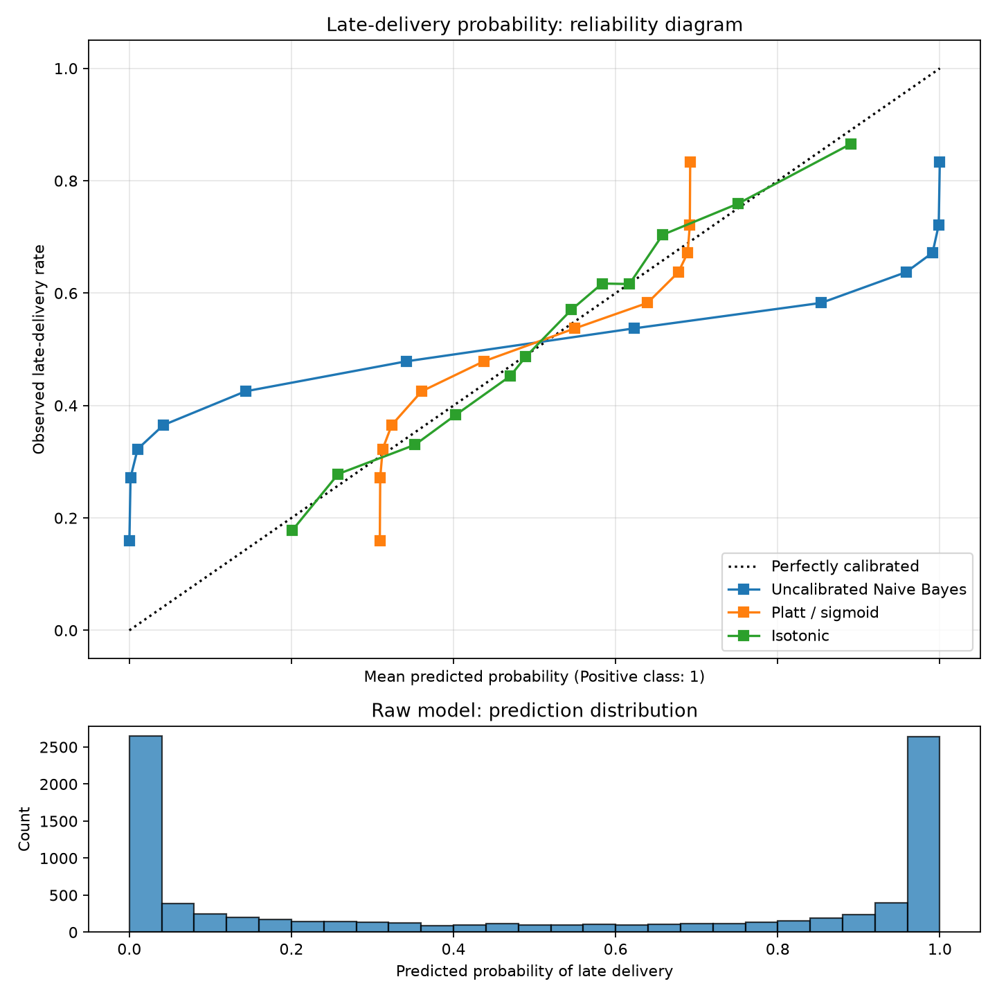
The upper plot compares the original and calibrated probability estimates.
The lower histogram shows how the original classifier distributes its predictions across the probability interval.
The diagonal reference line
A model following the diagonal has approximately matching predicted and observed event frequencies in each bin.
Curves far from the diagonal indicate calibration problems.
The original Gaussian Naive Bayes curve deviates substantially because the model assigns probabilities that are too extreme.
After calibration, the sigmoid and isotonic curves move substantially closer to the diagonal.
Why the histogram matters
A reliability diagram contains aggregated points.
Without the distribution of predictions, it is difficult to know how common particular probability ranges are.
For instance, a badly calibrated bin containing seven observations is not equivalent to a badly calibrated bin containing 70,000.
Both deserve investigation, but they have different statistical precision and operational impact.
Positive-class reliability versus top-label confidence
There is an important distinction in our evaluation.
The reliability diagram examines the predicted probability of late delivery, which is class 1.
The confidence-band report examines the probability assigned to whichever class the model predicts.
For binary classification:
confidence = max(p, 1 − p)
This means a prediction of 0.92 for late delivery and a prediction of 0.08 for late delivery both have 92% top-label confidence.
The latter is a 92% prediction of on-time delivery.
Our confidence-band accuracy calculation correctly includes both cases.
These are related but not identical calibration diagnostics.
9. Platt scaling: correcting scores with a sigmoid
Platt scaling learns a logistic transformation between a model’s outputs and observed event probabilities.
Conceptually, the transformation is:
p_calibrated = 1 / (1 + exp(−(a·s + b)))
Where:
-
s is an uncalibrated model score.
-
a controls the scale of the transformation.
-
b adjusts its offset.
-
p_calibrated is the corrected probability.
The parameters are learned from calibration data.
For estimators exposing probabilities, modern scikit-learn’s sigmoid calibration operates on their logit-transformed probability outputs. For estimators exposing only decision scores, the scores are used instead.
The practical goal is the same: learn a mapping from the original model output to observed event probability.
Why a sigmoid helps
Suppose your model produces probabilities that are consistently too extreme.
A sigmoid mapping can compress them toward the middle.
For example, a learned mapping might behave approximately like this:
| Raw probability | Calibrated probability |
|---|---|
| 0.02 | 0.24 |
| 0.15 | 0.34 |
| 0.50 | 0.50 |
| 0.85 | 0.66 |
| 0.98 | 0.76 |
These numbers are illustrative, not the exact mapping learned by our experiment.
Notice how the ordering is preserved.
Higher raw probabilities still receive higher calibrated probabilities.
The important change is their numerical interpretation.
Advantages
Platt scaling has several practical strengths:
-
It fits only a small number of parameters.
-
It is relatively data-efficient.
-
It produces a smooth mapping.
-
Its additional prediction cost is small.
-
A strictly increasing sigmoid mapping preserves the ranking of observations.
For a fixed binary score and a nondegenerate increasing sigmoid fit, ROC-AUC is therefore unchanged.
Limitations
Platt scaling cannot correct every possible calibration pattern.
It assumes a particular parametric relationship between scores and probabilities.
If the true calibration relationship is strongly irregular, asymmetric, or locally nonlinear, a sigmoid may remain systematically wrong.
It can also struggle when different regions of the score distribution require substantially different corrections.
That motivates a more flexible approach.
10. Isotonic regression: learn the shape from data
Isotonic regression learns a nondecreasing mapping from the model’s original outputs to observed event frequencies.
Unlike Platt scaling, it does not constrain the result to a sigmoid curve.
Instead, it finds a monotonic function that fits the calibration observations.
Conceptually:
p_calibrated = g(s)
The function g must be nondecreasing.
That means higher raw scores cannot receive lower calibrated probabilities.
However, the mapping is allowed to contain flat regions and irregular changes in slope.
Why monotonicity matters
Suppose the original classifier ranks order A above order B in predicted delay risk.
A monotonic calibrator respects that ordering in the sense that it cannot reverse it.
However, isotonic regression can assign both orders exactly the same calibrated probability.
This introduces ties.
As a result, isotonic calibration can change ROC-AUC slightly, even though the mapping never reverses a pair’s strict ordering.
Our experiment demonstrates this:
| Model | ROC-AUC |
|---|---|
| Uncalibrated | 0.7218 |
| Platt scaling | 0.7218 |
| Isotonic regression | 0.7212 |
The small decrease for isotonic regression comes from the effect of tied calibrated probabilities.
Why isotonic can outperform Platt scaling
Imagine a classifier with the following empirical relationship:
| Raw probability | Actual event frequency |
|---|---|
| 0.10 | 0.20 |
| 0.30 | 0.28 |
| 0.50 | 0.52 |
| 0.70 | 0.58 |
| 0.90 | 0.65 |
The relationship is monotonic, but it does not necessarily follow a convenient sigmoid shape.
Isotonic regression can adapt to that structure.
A sigmoid may leave noticeable residual errors.
The cost of flexibility
Isotonic regression is more prone to overfitting when calibration data is limited.
A small calibration dataset may produce a mapping with poorly estimated steps.
The scikit-learn documentation cautions against isotonic calibration with far fewer than approximately 1,000 calibration examples.
That is a practical guideline, not a universal threshold.
What matters is also the number of observations in the probability regions you care about.
A calibration set containing 10,000 observations can still provide weak evidence about probabilities above 0.99 if almost no predictions reach that range.
11. Choosing between Platt scaling and isotonic regression
The correct choice depends on the shape of miscalibration, calibration-sample size, and operational requirements.
| Consideration | Platt scaling | Isotonic regression |
|---|---|---|
| Calibration function | Parametric sigmoid | Nonparametric monotonic |
| Flexibility | Lower | Higher |
| Small calibration datasets | Usually more robust | Greater overfitting risk |
| Smooth output | Yes | Stepwise |
| Binary ranking preservation | Yes for increasing mapping | May introduce ties |
| Complex monotonic distortion | Limited | More adaptable |
| Typical inference overhead | Low | Low |
For many production systems, a reasonable approach is to start with sigmoid calibration and compare isotonic regression on a separate evaluation set.
Do not automatically choose isotonic because it achieves the lowest ECE on one dataset.
Instead, examine multiple metrics, their uncertainty, and the business importance of different probability ranges.
12. Measuring calibration: beyond reliability diagrams
Visual inspection is useful, but it is not enough.
We also need quantitative measurements.
Brier score
For binary classification, Brier score is the average squared difference between predicted probability and observed label.
Brier = mean((p − y)²)
Its value lies between 0 and 1 for binary outcomes, and smaller values are better.
It penalizes incorrect confident predictions heavily.
For example:
-
Predicting 0.90 when the outcome is 1 produces squared error 0.01.
-
Predicting 0.90 when the outcome is 0 produces squared error 0.81.
This makes it useful when probability errors have real decision consequences.
However, Brier score measures more than calibration alone.
It also reflects discrimination and the intrinsic uncertainty of the prediction problem.
A lower Brier score does not, by itself, prove that calibration improved.
Log loss
Log loss evaluates the probability assigned to the actual outcome.
It strongly penalizes highly confident incorrect predictions.
A model predicting 0.999 for an event that does not occur receives a very large penalty.
This sensitivity is valuable in applications where extreme probabilities drive consequential decisions.
It also means a few severe prediction errors can substantially affect the metric.
In our experiment, Platt scaling achieved slightly better log loss than isotonic regression, despite having a slightly worse Brier score.
Neither result is contradictory.
The metrics penalize probability errors differently.
Expected calibration error
Expected calibration error, or ECE, summarizes the differences between predicted probabilities and observed frequencies across bins.
A common binary positive-class formulation is:
ECE = sum over bins of (bin size / total size) × |observed frequency − mean predicted probability|
Our implementation uses 15 fixed-width probability bins.
It calculates the absolute calibration gap within each bin, weighted by that bin’s share of the observations.
In the experiment:
-
Uncalibrated ECE: approximately 0.243.
-
Platt ECE: approximately 0.036.
-
Isotonic ECE: approximately 0.020.
These results indicate substantial improvement in measured calibration.
Why ECE is not a perfect metric
ECE has several limitations.
First, its value depends on the binning strategy.
Changing the number of bins can change the result.
Second, averaging errors within bins can hide local variation.
A model might be overconfident for one subset and underconfident for another, with the deviations partially canceling before the absolute gap is calculated.
Third, empirical calibration estimates are noisy, particularly in sparse probability ranges.
Finally, ECE is not a strictly proper scoring rule. Optimizing it directly can encourage undesirable solutions.
Use ECE as a diagnostic rather than as the sole optimization objective.
For demanding applications, consider confidence intervals, adaptive binning, subgroup analysis, and more comprehensive probability-scoring evaluations.
13. Calibration without data leakage
One of the easiest ways to get misleading calibration results is to calibrate on the wrong data.
Consider this incorrect workflow:
-
Train a classifier on the full training dataset.
-
Predict probabilities on that same dataset.
-
Fit a calibrator using those predictions and labels.
-
Report calibration improvement on the same observations.
The calibrator is learning from predictions on data the classifier has already seen.
Those predictions can be unrealistically good.
The resulting probability mapping may become too extreme when applied to unfamiliar examples.
Correct option A: separate calibration dataset
This is the approach used in our experiment.
Train the original model on one dataset and fit the calibration mapping on another.
For a previously fitted scikit-learn estimator, FrozenEstimator prevents the base estimator from being refitted when passed into CalibratedClassifierCV.
The calibration dataset must be disjoint from the data used to fit the base model.
Correct option B: cross-validation calibration
When dedicated calibration data is unavailable, scikit-learn can use cross-validation to generate out-of-fold predictions for calibration.
The following self-contained example uses a synthetic classification dataset:
from sklearn.calibration import CalibratedClassifierCV
from sklearn.datasets import make_classification
from sklearn.model_selection import train_test_split
from sklearn.naive_bayes import GaussianNB
from sklearn.metrics import brier_score_loss

X, y = make_classification(
    n_samples=10_000,
    n_features=12,
    n_informative=5,
    n_redundant=5,
    random_state=42,
)

X_train, X_test, y_train, y_test = train_test_split(
    X,
    y,
    test_size=0.25,
    stratify=y,
    random_state=42,
)

model = CalibratedClassifierCV(
    estimator=GaussianNB(),
    method="sigmoid",
    cv=5,
    ensemble=False,
)

model.fit(X_train, y_train)

probabilities = model.predict_proba(X_test)[:, 1]

print(
    "Brier score:",
    brier_score_loss(y_test, probabilities),
)
With ensemble=False, cross-validation generates out-of-fold scores for learning the calibration mapping.
The final underlying estimator is then trained using the full training dataset.
This produces one base estimator plus its calibrator for prediction.
With ensemble=True, the system instead fits calibrated estimators across folds and averages their outputs during inference.
That can offer ensemble benefits, but it increases model size and prediction cost.
The current API uses ensemble="auto" by default, selecting behavior based on the estimator configuration.
See the scikit-learn CalibratedClassifierCV reference for the precise behavior.
14. Why calibration matters for business decisions
Imagine your logistics platform can expedite a shipment.
An intervention costs €5.
If an order would arrive late, expediting it successfully avoids a €25 penalty.
Assume, for this simplified example, that the intervention completely prevents the penalty and has no other effects.
The expected benefit of intervening is:
Expected avoided penalty = P(late) × €25
The intervention is economically justified when:
P(late) × €25 > €5
Therefore:
P(late) > 0.20
A 20% delay probability becomes the decision threshold.
Now consider a model that predicts 0.70 for an order whose true conditional late-delivery frequency is closer to 0.25.
The action may still be justified at the 20% threshold.
But the model substantially exaggerates expected savings.
This can distort resource allocation, budget forecasts, capacity planning, and the ranking of interventions.
If intervention capacity is constrained, ranking performance becomes important too.
This is why calibration and discrimination must be evaluated together.
Calibration improves the meaning of probabilities; it does not automatically improve the ranking of cases or guarantee better decisions.
15. Five advanced calibration pitfalls
1. Calibrating against the wrong population
Calibration learned on one population may fail on another.
Suppose you calibrate a delivery model using summer orders.
During winter, adverse weather increases the overall delay rate.
Even if feature distributions appear similar, the relationship between scores and outcomes may change.
A model calibrated for the summer population might now underestimate late-delivery risk.
Calibration does not automatically survive distribution shift.
Monitor it on recent, representative data.
2. Ignoring temporal structure
Random splitting is appropriate for our independent synthetic experiment.
It may be inappropriate for real production events.
For example, a shipping dataset collected over several years could have significant seasonality and operational drift.
A better evaluation may use:
-
Earlier observations for model training.
-
Later observations for calibration.
-
An even later period for final testing.
The exact split should mimic the data available when the model will be deployed.
Ensure that calibration never relies on labels that would not yet have been observed at the decision time.
3. Evaluating only global calibration
A globally calibrated model can be poorly calibrated within important subgroups.
Imagine two shipping regions.
In one region, the model consistently overestimates delays.
In the other, it consistently underestimates them.
The global reliability diagram might look acceptable if the errors cancel.
But local decisions remain unreliable.
Check calibration across operationally meaningful segments such as:
-
Delivery regions.
-
Shipping methods.
-
Order-value bands.
-
Forecast horizons.
-
Seasonal periods.
Avoid interpreting noisy subgroup results from tiny samples.
4. Assuming calibration improves accuracy
Post-hoc calibration primarily changes probability outputs.
It does not create new predictive information.
For a fixed binary classifier, a strictly increasing mapping preserves the ranking of examples.
It can still change classifications at a fixed probability threshold such as 0.5 if it shifts probabilities across that threshold.
Consequently, classification accuracy can rise, fall, or remain unchanged after calibration.
Reevaluate decision thresholds after calibrating.
Do not assume the original threshold remains optimal.
5. Assuming calibration is permanent
Suppose your model’s calibration is excellent immediately after deployment.
Six months later, operational processes change.
A new shipping partner improves average delivery performance.
Your original calibration mapping may no longer match observed outcomes.
A calibration model should therefore be treated as part of the production model pipeline.
It needs monitoring, validation, versioning, and periodic reassessment.
16. What about multiclass classification?
So far, our examples have involved a binary outcome: late or on-time delivery.
Multiclass classification introduces additional complexity.
Imagine predicting one of four delivery outcomes:
-
Early.
-
On time.
-
Slightly late.
-
Severely late.
The model outputs four probabilities that must sum to one.
Calibrating each class independently can produce values whose total differs from one.
Scikit-learn’s sigmoid and isotonic multiclass calibration handle this through a one-versus-rest approach followed by probability renormalization.
This makes the outputs usable as a probability distribution, although renormalization can interact with the individual class calibration mappings.
Modern scikit-learn also supports temperature scaling in CalibratedClassifierCV, introduced in version 1.8.
Temperature scaling adjusts model logits using a learned temperature parameter before converting them into probabilities.
For multiclass models, it is particularly attractive because it operates naturally on the joint class-probability distribution.
Its limited parameterization can also make it easier to fit with smaller calibration sets, although it cannot correct arbitrary class-specific errors.
When evaluating multiclass calibration, distinguish between:
-
Classwise calibration: Whether each class’s predicted probabilities match observed frequencies.
-
Top-label calibration: Whether the predicted class’s confidence matches its accuracy.
-
Joint probability quality: Whether the entire predicted distribution is useful under a proper scoring rule.
A single top-label reliability diagram cannot establish that the full multiclass distribution is calibrated.
17. A production-ready calibration workflow
A robust calibration system is more than a call to a calibration API.
The process should cover data quality, experiment design, deployment, and monitoring.
Before calibration
-
Confirm that the base model has useful discrimination.
-
Check whether probabilities are overconfident, underconfident, or distorted in more complicated ways.
-
Build reliability diagrams using representative evaluation data.
-
Inspect sample counts in important probability ranges.
-
Establish baseline Brier score, log loss, and ECE.
During calibration
-
Keep model-training and calibration observations separate.
-
Compare sigmoid and isotonic mappings.
-
Use cross-validation when a dedicated calibration set is impractical.
-
Avoid fitting or selecting methods using the final test set.
-
Preserve preprocessing and feature transformations exactly as used by the base model.
After calibration
-
Evaluate on a genuinely untouched dataset.
-
Compare proper scoring rules, not only ECE.
-
Check whether rankings or decision thresholds have changed.
-
Evaluate important operational subgroups.
-
Measure the cost and benefit of calibrated decisions.
-
Save the base estimator and calibration mapping together.
-
Monitor calibration drift after deployment.
One subtle operational point is worth emphasizing: calibration depends on the distribution of predictions from a particular model version.
If you retrain the base model, its score distribution can change.
Do not assume a calibrator trained for the previous model version remains valid.
Validate or refit it as part of the updated model pipeline.
18. When calibration is not enough
Calibration is powerful, but it cannot repair every model problem.
Suppose your classifier cannot distinguish difficult orders from easy ones.
Its ROC-AUC is approximately 0.5.
A calibrator might still transform its outputs into probabilities that match aggregate event frequencies.
But the result does not suddenly become a useful ranking system.
Similarly, if the base model systematically lacks important explanatory variables, calibration cannot recover information that was never present in its scores.
Calibration corrects the interpretation of a model’s existing output.
It does not generally solve:
-
Missing predictive features.
-
Incorrect or inconsistent labels.
-
Severe data leakage.
-
Poor class separation.
-
Unrepresentative training examples.
-
Fundamental changes in the underlying prediction problem.
A sensible sequence is to establish useful discrimination, diagnose probability quality, calibrate where needed, and then evaluate the resulting decisions.
19. Key lessons from the experiment
We began with a classifier that seemed confident.
It routinely assigned probabilities close to 0 or 1.
Its ROC-AUC showed that it contained meaningful predictive information.
But for predictions averaging 90.7% top-label confidence, observed accuracy was only 61.1%.
The problem was not simply that the model made mistakes.
The deeper problem was that its probability scale was wrong.
By fitting calibration mappings on independent data, we substantially improved the reliability of those probabilities.
The experiment also highlighted several important distinctions:
-
Platt scaling can correct confidence distortions with a simple, smooth transformation.
-
Isotonic regression offers greater flexibility but needs sufficient calibration data.
-
Better calibration does not necessarily mean better ranking.
-
Different proper scoring rules can prefer different calibrated models.
-
Independent evaluation is necessary to establish whether calibration generalizes.
-
Probability quality must be monitored as the production environment evolves.
Most importantly, a prediction of 90% should carry a meaningful statistical interpretation.
If it does not, downstream systems are making decisions using numbers that appear more precise than they really are.
Further reading
These references document the APIs and practical methods used throughout this tutorial:
-
scikit-learn: Probability calibration user guide — theoretical foundations, reliability diagrams, and calibration techniques.
-
CalibratedClassifierCV API — current sigmoid, isotonic, temperature-scaling, and cross-validation options.
-
CalibrationDisplay API — reliability-diagram visualization.
-
FrozenEstimator API — calibrating previously fitted estimators without refitting them.
Your next step: audit the probabilities you already trust
Run the experiment, generate the reliability diagram, and observe how dramatically the confidence distribution changes after calibration.
Then take a classifier from one of your own non-sensitive projects and perform the same evaluation.
Start by collecting its predicted probabilities and actual outcomes on untouched data. Compute Brier score and log loss, draw a reliability diagram, and compare sigmoid and isotonic calibration using an appropriate validation strategy.
Pay particular attention to the probability ranges where real decisions happen.
A model that predicts the correct class is useful. A model that also knows how uncertain it is can be substantially more valuable.
Before trusting your next 90% prediction, measure what 90% actually means.