
LEARN · CLASSICAL MACHINE LEARNING
1. Why regularization is a diagnostic problem, not just a tuning problem
A machine learning model can fail in two opposite ways.
It can be too simple to capture meaningful relationships in the data. Or it can become so flexible that it learns accidental patterns in the training sample rather than relationships that generalize.
These failures are commonly called underfitting and overfitting.
Regularization helps control the second problem by discouraging unnecessary model complexity. But applying more regularization is not automatically better.
Too little regularization can produce unstable predictions. Too much can prevent the model from learning useful signals.
The practical challenge is therefore not merely finding a regularization parameter that produces a good validation score. It is understanding why that parameter works, how much uncertainty surrounds the selection, and whether the answer will change as the dataset grows.
In this tutorial, we will build a complete diagnostic workflow using scikit-learn:
-
Construct a reproducible regression dataset with nonlinear relationships.
-
Sweep regularization strengths and compare training against validation error.
-
Generate learning curves that reveal how performance changes with sample size.
-
Recognize four important diagnostic patterns.
-
Select a simpler model using the one-standard-error rule.
-
Investigate how the preferred regularization strength changes when more training data becomes available.
-
Transfer the same reasoning to boosted trees and neural networks.
We will also examine a surprising example where adding enough data makes an unregularized model outperform every regularized alternative.
The guiding principle is simple:
Choose regularization by observing generalization behavior, not by treating a hyperparameter value as intrinsically good or bad.
2. The mechanics: what does regularization actually change?
Most supervised learning algorithms optimize a loss function measuring how poorly predictions match their targets.
Regularization adds another consideration: the complexity of the model.
A generic objective looks like this:
Objective = Training loss + λ × Complexity penalty
Here, λ controls how strongly complexity is penalized.
-
When λ is small, the model prioritizes fitting the training data.
-
When λ is large, the model sacrifices some training accuracy to remain simpler.
-
When λ is zero, the explicit penalty disappears.
This creates a trade-off between fitting the observed data and producing stable predictions on future examples.
L2 regularization: shrinking coefficients
Ridge regression uses an L2 penalty: the sum of squared model coefficients.
For scikit-learn’s Ridge, the objective is:
Objective = Σ(yᵢ − ŷᵢ)² + α × Σwⱼ²
Here:
-
yᵢis an observed target. -
ŷᵢis the prediction. -
wⱼis a model coefficient. -
αcontrols regularization strength.
As alpha increases, large coefficients become more expensive.
This often reduces sensitivity to correlated features and noise.
Importantly, Ridge generally shrinks coefficients toward zero without making them exactly zero.
L1 regularization: encouraging sparsity
Lasso regression instead penalizes the sum of absolute coefficient values.
Its penalty is proportional to:
α × Σ|wⱼ|
This encourages some coefficients to become exactly zero, effectively performing feature selection.
L1 and L2 penalties solve related but different problems.
L1 is useful when sparse solutions are desirable. L2 is often attractive when many features contain weak but useful signals.
There is also Elastic Net, which combines both approaches.
An important implementation detail: scikit-learn does not normalize the data-fitting term identically across all estimators.
For example, Ridge uses a sum of squared residuals, while Lasso scales its squared-error term by the number of samples.
Consequently, identical numeric alpha values do not imply equivalent regularization across estimators.
The current scikit-learn linear-model documentation describes these objectives precisely.
3. The train-versus-validation gap is the central diagnostic
Imagine evaluating three regression models using root mean squared error (RMSE).
Lower values are better.
| Model | Training RMSE | Validation RMSE | Gap |
|---|---|---|---|
| A | 1.0 | 3.4 | 2.4 |
| B | 1.5 | 1.8 | 0.3 |
| C | 4.1 | 4.2 | 0.1 |
Model A fits training data extremely well, but its validation performance is substantially worse.
That large gap suggests high variance: the model has learned patterns that do not transfer reliably.
Model C has almost no gap. However, both errors are high.
This is a classic underfitting pattern.
Model B has moderately low training and validation errors with a relatively small gap.
It is the strongest candidate of the three.
The gap is:
Generalization gap = Validation error − Training error
For an error metric such as RMSE, a large positive gap is a warning sign.
But notice the crucial distinction:
A small gap does not prove that the model is good. It only suggests that training and validation performance are similar.
A useless model can perform equally badly on both datasets.
That is why regularization diagnostics must inspect both the absolute error and the gap.
Also remember that the gap is affected by evaluation design. The training score is calculated on samples used to fit the model, whereas the validation score comes from held-out samples. Differences in sample sizes, noise, distribution, and scoring procedures all influence the observed gap.
The gap is evidence, not a mathematical measurement of variance by itself.
4. Building a reproducible experiment
We will use a synthetic retail order-value prediction problem.
The features represent five normalized order characteristics. The target follows a mixture of linear effects, nonlinear effects, interactions, and random noise.
This is useful because it gives us a controlled environment where both excessive flexibility and excessive regularization can cause problems.
Our model will combine:
-
Polynomial feature expansion.
-
Standardization.
-
Ridge regression.
The polynomial expansion creates enough flexibility for the model to overfit. Ridge gives us a way to control that flexibility.
Step 1: Set up the environment
The code targets scikit-learn 1.9.1, the stable release available in October 2026.
Create a virtual environment and install the dependencies:
python -m venv .venv
source .venv/bin/activate
python -m pip install "scikit-learn==1.9.1" "numpy>=2.0" "matplotlib>=3.9"
The activation command above is for Unix-like shells. On Windows, use the activation command appropriate to your shell.
We will use the current validation_curve, learning_curve, GridSearchCV, and root_mean_squared_error APIs.
Step 2: Implement the complete diagnostic experiment
Save the following program as regularization_lab.py.
It generates the dataset, computes both diagnostic curves, applies the one-standard-error rule, checks sample-size effects, saves a plot, and evaluates the selected model against an untouched test set.
import numpy as np
import matplotlib.pyplot as plt

from sklearn.base import clone
from sklearn.linear_model import Ridge
from sklearn.metrics import root_mean_squared_error
from sklearn.model_selection import (
    GridSearchCV,
    KFold,
    learning_curve,
    train_test_split,
    validation_curve,
)
from sklearn.pipeline import make_pipeline
from sklearn.preprocessing import PolynomialFeatures, StandardScaler


# --------------------------------------------------
# 1. Generate synthetic retail order data
# --------------------------------------------------

rng = np.random.default_rng(17)

X = rng.uniform(-1.5, 1.5, size=(680, 5))

y = (
    10
    + 4.0 * X[:, 0]
    - 2.5 * X[:, 1]
    + 2.0 * X[:, 2] ** 2
    + 1.4 * X[:, 0] * X[:, 1]
    + 1.2 * np.sin(1.7 * X[:, 3])
    + rng.normal(0, 1.4, size=len(X))
)

X_train, X_test, y_train, y_test = train_test_split(
    X,
    y,
    test_size=0.25,
    random_state=31,
)


# --------------------------------------------------
# 2. Build a leakage-safe modeling pipeline
# --------------------------------------------------

estimator = make_pipeline(
    PolynomialFeatures(
        degree=4,
        include_bias=False,
    ),
    StandardScaler(),
    Ridge(solver="cholesky"),
)

cv = KFold(
    n_splits=5,
    shuffle=True,
    random_state=23,
)

alphas = np.logspace(-3, 4, 12)


# --------------------------------------------------
# 3. Calculate the regularization validation curve
# --------------------------------------------------

train_scores, valid_scores = validation_curve(
    estimator,
    X_train,
    y_train,
    param_name="ridge__alpha",
    param_range=alphas,
    cv=cv,
    scoring="neg_root_mean_squared_error",
    n_jobs=1,
)

# scikit-learn returns negative errors for maximization.
train_rmse = -train_scores
valid_rmse = -valid_scores

train_mean = train_rmse.mean(axis=1)
valid_mean = valid_rmse.mean(axis=1)

best_idx = int(np.argmin(valid_mean))
best_alpha = float(alphas[best_idx])


# --------------------------------------------------
# 4. Apply the one-standard-error rule
# --------------------------------------------------

best_standard_error = (
    valid_rmse[best_idx].std(ddof=1)
    / np.sqrt(valid_rmse.shape[1])
)

threshold = valid_mean[best_idx] + best_standard_error

eligible = np.flatnonzero(valid_mean <= threshold)

# Larger Ridge alpha means stronger regularization.
one_se_idx = int(eligible[-1])
one_se_alpha = float(alphas[one_se_idx])

print("Minimum-CV-error alpha:", round(best_alpha, 4))
print("One-SE alpha:", round(one_se_alpha, 4))
print("Best CV RMSE:", round(valid_mean[best_idx], 4))
print("One-SE CV RMSE:", round(valid_mean[one_se_idx], 4))


# --------------------------------------------------
# 5. Generate a learning curve
# --------------------------------------------------

selected_estimator = clone(estimator).set_params(
    ridge__alpha=one_se_alpha
)

sizes, lc_train_scores, lc_valid_scores = learning_curve(
    selected_estimator,
    X_train,
    y_train,
    train_sizes=[0.12, 0.25, 0.5, 0.75, 1.0],
    cv=cv,
    scoring="neg_root_mean_squared_error",
    shuffle=True,
    random_state=19,
    n_jobs=1,
)

lc_train = -lc_train_scores
lc_valid = -lc_valid_scores

lc_train_mean = lc_train.mean(axis=1)
lc_valid_mean = lc_valid.mean(axis=1)


# --------------------------------------------------
# 6. Draw both diagnostic curves
# --------------------------------------------------

fig, axes = plt.subplots(1, 2, figsize=(13, 5))

axes[0].semilogx(
    alphas,
    train_mean,
    marker="o",
    label="Training RMSE",
)

axes[0].semilogx(
    alphas,
    valid_mean,
    marker="o",
    label="Validation RMSE",
)

axes[0].fill_between(
    alphas,
    valid_mean - valid_rmse.std(axis=1),
    valid_mean + valid_rmse.std(axis=1),
    alpha=0.15,
)

axes[0].axvline(
    best_alpha,
    linestyle="--",
    label="Minimum CV error",
)

axes[0].axvline(
    one_se_alpha,
    linestyle=":",
    label="One-SE choice",
)

axes[0].set_xlabel("Ridge alpha")
axes[0].set_ylabel("RMSE")
axes[0].set_title("Validation curve")
axes[0].legend()
axes[0].grid(True, alpha=0.3)

axes[1].plot(
    sizes,
    lc_train_mean,
    marker="o",
    label="Training RMSE",
)

axes[1].plot(
    sizes,
    lc_valid_mean,
    marker="o",
    label="Validation RMSE",
)

axes[1].fill_between(
    sizes,
    lc_valid_mean - lc_valid.std(axis=1),
    lc_valid_mean + lc_valid.std(axis=1),
    alpha=0.15,
)

axes[1].set_xlabel("Training-set size")
axes[1].set_ylabel("RMSE")
axes[1].set_title("Learning curve")
axes[1].legend()
axes[1].grid(True, alpha=0.3)

plt.tight_layout()

plt.savefig(
    "regularization_diagnostics.png",
    dpi=160,
    bbox_inches="tight",
)

plt.close(fig)


# --------------------------------------------------
# 7. Re-tune alpha at different dataset sizes
# --------------------------------------------------

order = np.random.default_rng(2026).permutation(len(X_train))

fine_alphas = np.logspace(-3, 4, 22)

print("\nTraining size | Best alpha | Alpha / size")

for count in [90, 300, len(X_train)]:
    indices = order[:count]

    search = GridSearchCV(
        estimator,
        param_grid={"ridge__alpha": fine_alphas},
        cv=cv,
        scoring="neg_root_mean_squared_error",
        n_jobs=1,
    )

    search.fit(
        X_train[indices],
        y_train[indices],
    )

    alpha = float(search.best_params_["ridge__alpha"])

    print(
        f"{count:13d} | "
        f"{alpha:10.4f} | "
        f"{alpha / count:12.5f}"
    )


# --------------------------------------------------
# 8. Evaluate the selected model once
# --------------------------------------------------

selected_estimator.fit(X_train, y_train)

predictions = selected_estimator.predict(X_test)

test_rmse = root_mean_squared_error(
    y_test,
    predictions,
)

print("\nFinal test RMSE:", round(test_rmse, 4))
print("Saved regularization_diagnostics.png")
Execute it:
python regularization_lab.py
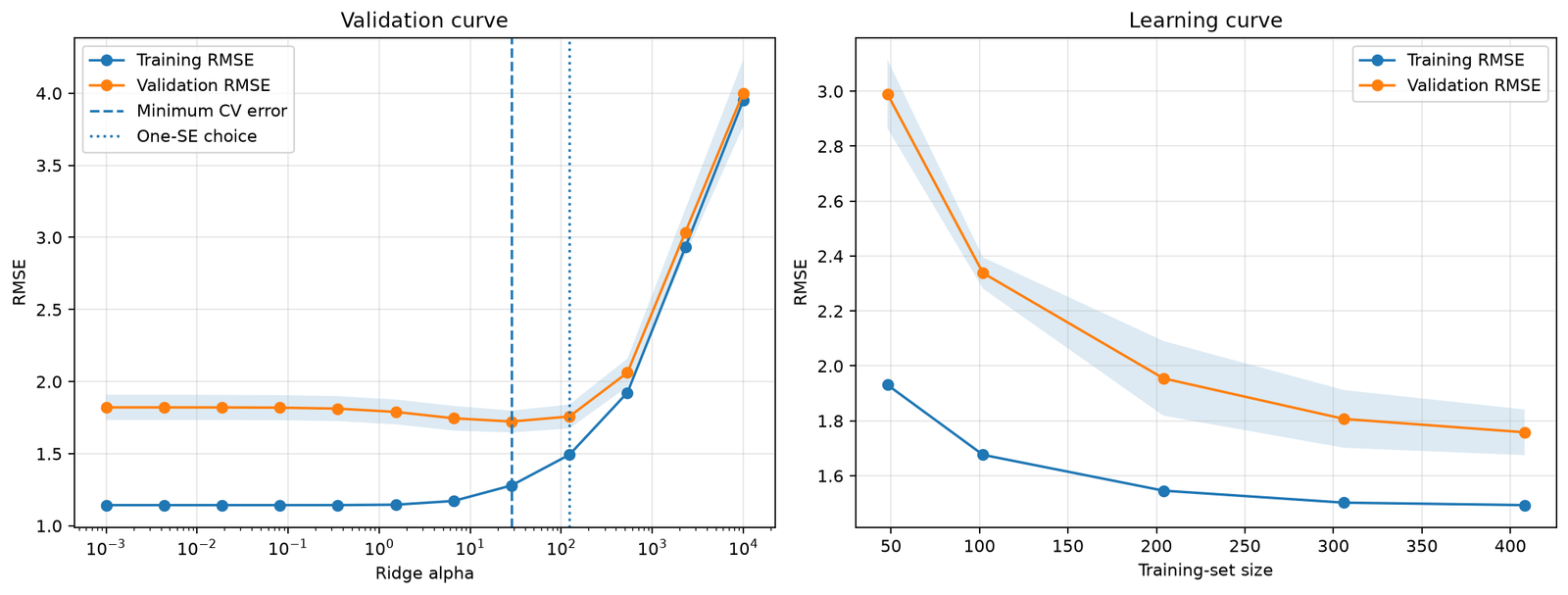
The script produces two curves in regularization_diagnostics.png, along with the selected regularization values and a final held-out test score.
Our run (scikit-learn 1.9.1) produced this figure:
The experiment is entirely reproducible because dataset generation, splitting, and sampling use fixed random seeds.
Why the pipeline matters
Notice that polynomial expansion and standardization live inside the scikit-learn pipeline.
This is intentional.
During cross-validation, the pipeline fits its transformations separately within each training fold.
It does not estimate scaling statistics from the validation fold.
Preprocessing the entire dataset before cross-validation would expose validation-distribution information to the training procedure and could bias the estimate of generalization performance.
The same principle applies to imputation, feature selection, dimensionality reduction, and target-aware transformations.
All learned preprocessing belongs inside the cross-validation pipeline.
5. Reading a validation curve: how much regularization is enough?
A validation curve changes one hyperparameter while holding the other modeling choices constant.
In our experiment, the parameter is Ridge alpha.
The horizontal axis represents regularization strength. The vertical axis represents prediction error.
Typically, the training error increases as regularization becomes stronger.
The validation error may initially fall because regularization reduces overfitting, then rise because excessive regularization introduces too much bias.
That produces a roughly U-shaped validation-error curve.
What the experiment shows
With the generated data and selected cross-validation configuration, representative results are:
| Ridge alpha | Training RMSE | Validation RMSE | Gap |
|---|---|---|---|
| 0.001 | 1.143 | 1.821 | 0.678 |
| 28.48 | 1.280 | 1.723 | 0.443 |
| 123.28 | 1.493 | 1.758 | 0.265 |
| 10,000 | 3.951 | 4.001 | 0.050 |
These numbers tell a useful story.
At alpha = 0.001, the model performs much better on training data than on validation data.
The gap of approximately 0.68 indicates substantial generalization deterioration.
Increasing alpha to approximately 28.48 raises the training error slightly but improves validation performance.
This is precisely what useful regularization should accomplish.
At alpha = 123.28, the gap becomes smaller still. Validation error is a little worse than at the minimum, but the model is more strongly constrained.
Finally, at alpha = 10,000, both errors are high.
The model is no longer capturing the underlying relationships adequately.
The three regions of the curve
Conceptual validation curve, not the exact output of the experiment. Lower error is better; the optimum lies between overfitting and underfitting.Region 1: Insufficient regularization. Training error is relatively low, but validation error is much higher. Strengthening regularization may reduce the gap and improve generalization.
Region 2: Useful regularization. Validation error approaches its minimum. This is where we should investigate model stability and uncertainty rather than blindly picking the lowest observed point.
Region 3: Excessive regularization. Both training and validation errors rise. The model is losing the flexibility needed to represent the data.
The exact curve need not be smooth or U-shaped. Real datasets can produce irregular curves, multiple near-optimal regions, or an optimum at the edge of the search range.
When the best result is at a boundary, expand the search in that direction before drawing conclusions.
6. Learning curves: distinguishing model problems from data problems
A validation curve varies regularization strength.
A learning curve varies the amount of training data.
These are complementary diagnostics.
A typical learning curve plots:
-
Training performance as the number of training examples increases.
-
Cross-validated performance on held-out examples at each training size.
The validation fold should remain separate from the subsample used for fitting.
In our script, learning_curve handles these splits.
At each requested training size, it fits models on subsets of the available training folds.
The code fixes alpha at the previously selected one-standard-error value. This means the learning curve describes the behavior of that particular regularization setting, not a model retuned separately at every size.
That distinction matters: a learning curve for a fixed estimator and a learning curve for an entire hyperparameter-selection procedure answer different questions.
Four shapes every practitioner should recognize
| Pattern | Training error | Validation error | Interpretation |
|---|---|---|---|
| High bias | High | High and close to training | Model cannot adequately fit the signal |
| High variance | Low | Much higher than training | Model is sensitive to the training sample |
| Converged, good fit | Low | Low and close to training | Model generalizes reasonably well |
| Not enough data | Often low or moderate | Still improving as data grows, often with a persistent gap | More observations may improve generalization |
Shape 1: High bias
Both curves remain at relatively high error levels and approach each other.
For example, training RMSE might stabilize around 4.0 and validation RMSE around 4.2.
Adding more data may produce little improvement because the model already fails to fit its existing training data.
Potential remedies include:
-
Reducing overly strong regularization.
-
Increasing model capacity.
-
Introducing relevant nonlinear features or interactions.
-
Improving the feature representation.
-
Checking whether the chosen model family can represent the target relationship.
A linear model cannot represent a strongly nonlinear signal merely because we collect more observations.
It needs features or architecture capable of representing that signal.
Shape 2: High variance
Training error remains much lower than validation error.
The gap may gradually narrow as training size increases.
For example, training RMSE might be 0.9 while validation RMSE is 2.8.
Potential remedies include:
-
Increasing regularization.
-
Reducing model complexity.
-
Removing unstable or irrelevant features.
-
Gathering more representative training samples.
-
Using more robust preprocessing or data-quality controls.
If the validation curve strongly improves when alpha increases, stronger regularization is an especially plausible intervention.
If the learning curve shows a narrowing gap and improving validation results as training size grows, more data may help substantially.
Shape 3: Converged with a good fit
Training and validation errors meet near an acceptably low value.
For example, they may stabilize around 1.5 and 1.6.
This usually suggests that additional training samples will offer diminishing returns under the current distribution and model configuration.
At this stage, improving the system may require better features, a lower noise floor, or a more suitable modeling objective.
But convergence alone does not guarantee good performance. The absolute error must still be evaluated against a baseline and business requirements.
Shape 4: Not enough data
The validation error is still declining at the largest available training size, and the gap has not stabilized.
That indicates that additional observations could improve performance.
For example:
-
With 100 examples, validation RMSE is 3.2.
-
With 300 examples, it is 2.4.
-
With 700 examples, it is 1.9.
-
At the right edge of the curve, it is still trending downward.
That is a stronger argument for collecting data than a generic assumption that more data is always beneficial.
However, a rising-performance trend is not proof that data quantity is the only problem.
A distribution shift, labeling inconsistency, or poor feature representation can also influence the curves.
The learning curve supports a decision; it does not establish causality.
Interpreting our generated learning curve
The selected model produces approximately the following average values at the smallest and largest sampled sizes:
| Training examples used per fold | Training RMSE | Validation RMSE |
|---|---|---|
| 48 | 1.93 | 2.99 |
| 408 | 1.49 | 1.76 |
Notice what happens.
As the training set grows, the training error decreases in this particular experiment, while validation error falls substantially.
Although training error often rises with sample size in idealized learning-curve diagrams, monotonic behavior is not guaranteed for every regularized model or sampled dataset.
Here the learning-curve trend indicates that additional data helps the selected model learn its nonlinear relationships more reliably.
The remaining gap also suggests that the model has not completely eliminated variance-related behavior.
7. The one-standard-error rule: preferring a simpler model without chasing tiny differences
A hyperparameter sweep often produces several models with nearly identical validation performance.
Consider two configurations:
-
Model A has validation RMSE of 1.72.
-
Model B has validation RMSE of 1.76.
Model A has the smaller observed error.
But does this tiny difference justify selecting the more flexible model?
Not necessarily.
Cross-validation scores vary because different folds contain different observations.
The one-standard-error rule provides a practical way to select a simpler model when its estimated performance is sufficiently close to the optimum.
How the rule works
For an error metric, the procedure is:
-
Identify the configuration with the lowest mean cross-validation error.
-
Estimate the standard error of that configuration’s fold-level error scores.
-
Add one standard error to the minimum mean error.
-
Identify every configuration whose mean error is below that threshold.
-
Select the simplest eligible configuration.
In our Ridge experiment, simplicity means stronger coefficient shrinkage, so we choose the largest eligible alpha.
The estimated standard error is:
SE = Sample standard deviation of fold errors / √k
Here, k is the number of validation folds.
This is a useful heuristic, not a formal guarantee of equivalence. Cross-validation folds share training observations, and their results are not independent in the way required by a simple confidence-interval calculation.
Worked example
The lowest average validation RMSE in our sweep is approximately:
Best RMSE = 1.723
The estimated standard error is approximately:
SE = 0.038
Therefore:
Eligibility threshold = 1.723 + 0.038 = 1.761
Every configuration with mean validation RMSE no greater than approximately 1.761 qualifies.
The strongest regularization setting that qualifies is:
Alpha ≈ 123.28
This contrasts with the minimum-error choice:
Alpha ≈ 28.48
The one-standard-error choice accepts a small increase in estimated error in exchange for stronger coefficient shrinkage.
That is not a claim that alpha 123.28 is objectively better.
It is an explicit preference for a more constrained model when the available validation evidence does not show a large penalty for that preference.
When should you use it?
The rule is particularly attractive when:
-
Model stability matters more than squeezing out tiny validation gains.
-
The validation curve has a broad, flat optimum.
-
The training-versus-validation gap remains substantial.
-
A modest loss in predictive accuracy is acceptable in exchange for lower complexity.
For other model families, the simplicity ordering must be defined appropriately.
For example, a shallower decision tree is generally simpler than a deeper one. A neural network with heavier weight decay may be more constrained, but parameter magnitude alone does not fully characterize its effective complexity.
The rule also depends on the candidate grid. A different search range or resolution can change which models qualify.
8. Why the best alpha can shift as the dataset grows
Regularization strength should not automatically remain fixed when the dataset expands.
With a small dataset, flexible estimators may learn many accidental correlations.
As the number of observations increases, those relationships can become easier to distinguish from genuine signals.
This frequently reduces the relative amount of regularization needed.
But there is an implementation detail that makes the story more interesting.
Ridge alpha is not normalized by sample count
Recall scikit-learn’s Ridge objective:
Σ(yᵢ − ŷᵢ)² + α × Σwⱼ²
The data-fitting term sums across observations.
Adding more observations changes the scale of that term.
If we divide the entire objective by the number of observations, the equivalent expression is:
Mean squared error + (α / n) × Σwⱼ²
This reveals that the effective penalty relative to average loss is governed by alpha divided by the number of training samples.
Consequently:
-
A fixed raw Ridge alpha becomes relatively weaker as n increases.
-
Holding alpha/n constant requires raw alpha to grow proportionally with n.
-
The best raw alpha can increase, decrease, or remain similar as data grows.
This is why assuming that the best Ridge alpha must monotonically decrease with training size is incorrect.
Demonstrating the shift
The script retunes alpha using 90, 300, and 510 development-set observations.
For the seeded experiment, the finer grid produces approximately:
| Training observations | Best raw alpha | Alpha / n |
|---|---|---|
| 90 | 21.54 | 0.239 |
| 300 | 46.42 | 0.155 |
| 510 | 21.54 | 0.042 |
The raw alpha does not decrease monotonically.
It increases and then decreases.
But the penalty relative to training-set size becomes substantially smaller overall.
The comparison is approximate because the actual cross-validation fits use only the training portion of each fold, not all n observations in the subset.
Still, it demonstrates the essential principle.
When comparing Ridge regularization across dataset sizes, inspect the scale of the objective and the effective penalty, not only the raw alpha value.
There is an additional reason to retune after significant dataset growth: the best hyperparameters may change because the estimator sees more of the feature distribution.
New observations can improve coefficient estimates, expose rare feature combinations, change feature-selection reliability, or reveal previously hidden nonlinearities.
The right response is periodic re-evaluation, not an automatic alpha adjustment.
9. Transferring the skill across model families
Regularization is not unique to linear regression.
Many popular algorithms expose controls that reduce overfitting, although they operate in different ways.
The central diagnostic remains the same: compare training performance against validation performance while varying model complexity or regularization strength.
| Model family | Regularization controls | Direction toward a more constrained model | Important distinction |
|---|---|---|---|
| Ridge regression | alpha |
Increase alpha | Shrinks coefficients using L2 |
| Lasso regression | alpha |
Increase alpha | Encourages sparse coefficients using L1 |
| Elastic Net | alpha, l1_ratio |
Increase alpha for a fixed mixing ratio | Combines L1 and L2 penalties |
| Logistic regression | C |
Decrease C | C is inverse regularization strength |
| XGBoost tree boosting | reg_lambda, reg_alpha |
Increase penalty | Penalizes leaf weights |
| XGBoost tree boosting | gamma |
Increase gamma | Requires greater loss reduction before splitting |
| Neural networks | weight_decay |
Increase weight decay | Discourages large parameter values |
| Neural networks | Dropout probability | Increase dropout moderately | Randomly masks activations during training |
The parameters in this table are not numerically interchangeable.
For example, increasing gamma in XGBoost changes whether proposed tree splits are accepted, while increasing reg_lambda penalizes leaf weights.
Likewise, neural-network dropout is a stochastic training mechanism, not simply another coefficient penalty.
The current XGBoost parameter documentation distinguishes reg_lambda, reg_alpha, and gamma. PyTorch’s AdamW documentation describes decoupled weight decay.
Example: diagnosing gradient-boosted trees
Suppose a boosted-tree model has excellent training accuracy but much worse validation accuracy.
A useful sequence is:
-
Increase
reg_lambdato constrain leaf weights. -
Increase
gammato discourage low-value splits. -
Limit tree depth or increase minimum child requirements.
-
Adjust the number of boosting rounds and learning rate together.
-
Consider row or feature subsampling.
Then regenerate the validation curve for the relevant parameter.
Do not increase all constraints simultaneously at first. That would make it difficult to determine which change actually helped.
Example: diagnosing neural networks
Suppose training loss keeps falling while validation loss begins rising.
Potential interventions include:
-
Increasing weight decay.
-
Introducing or increasing dropout.
-
Reducing network capacity.
-
Using early stopping.
-
Increasing the quantity or diversity of representative training data.
A validation curve can be produced by repeatedly training the network with different weight-decay values.
A learning curve can be produced by retraining it on increasingly large subsets of the dataset.
Neural networks introduce additional complications, including optimization randomness, learning-rate schedules, batch size, and training duration.
To isolate regularization effects, control these variables as carefully as possible.
In particular, a model that has not trained long enough may look underfit even when its capacity and regularization are appropriate.
10. The cherry on the cake: more data can eliminate the need for explicit regularization
Here is a surprising case.
We will generate a noiseless linear regression problem with 32 correlated features.
Only three coefficients actually contribute to the target.
First, we train using just 12 examples.
That is an underdetermined problem: there are more features than training observations.
Then we train using 800 examples.
The underlying data-generating relationship remains exactly the same.
Because the target is a noiseless linear combination of the available features, ordinary least squares can eventually recover the relationship to numerical precision once the system has sufficient independent information.
Runnable experiment
import numpy as np

from sklearn.linear_model import LinearRegression, Ridge
from sklearn.metrics import root_mean_squared_error


rng = np.random.default_rng(1)

n_features = 32

# Create correlated tabular features.
mixing = rng.normal(size=(n_features, n_features))

X = (
    rng.normal(size=(2200, n_features))
    @ mixing
    / np.sqrt(n_features)
)

# The true process depends on only three features.
true_coefficients = np.zeros(n_features)
true_coefficients[:3] = [3.0, -2.0, 1.0]

# Noiseless target.
y = X @ true_coefficients

# Independent evaluation portion.
X_eval = X[-1000:]
y_eval = y[-1000:]

alphas = [0, 0.01, 0.1, 1, 10, 100]

for train_count in [12, 800]:
    print(f"\nTraining examples: {train_count}")

    results = []

    for alpha in alphas:
        if alpha == 0:
            model = LinearRegression()
        else:
            model = Ridge(alpha=alpha)

        model.fit(
            X[:train_count],
            y[:train_count],
        )

        predictions = model.predict(X_eval)

        rmse = root_mean_squared_error(
            y_eval,
            predictions,
        )

        results.append((alpha, rmse))

        print(
            f"alpha={alpha:7.2f} "
            f"RMSE={rmse:.6f}"
        )

    best_alpha, best_rmse = min(
        results,
        key=lambda item: item[1],
    )

    print(
        f"Best observed alpha: {best_alpha}"
    )
We use LinearRegression for the zero-regularization case, rather than passing zero to Ridge. This follows scikit-learn’s recommendation for ordinary least squares.
Results
With 12 training examples:
| Alpha | Evaluation RMSE |
|---|---|
| 0 | 2.3324 |
| 0.01 | 2.3309 |
| 0.1 | 2.3178 |
| 1 | 2.2167 |
| 10 | 2.1371 |
| 100 | 2.7142 |
The smallest evaluation error in this illustrative grid occurs at alpha = 10.
A modest amount of regularization improves predictions when there are too few observations to identify the relevant coefficient structure reliably.
Now consider 800 training examples:
| Alpha | Evaluation RMSE |
|---|---|
| 0 | Approximately 0 |
| 0.01 | 0.0004 |
| 0.1 | 0.0034 |
| 1 | 0.0158 |
| 10 | 0.1033 |
| 100 | 0.5328 |
The unregularized model now performs best.
It recovers the noiseless generating relationship to numerical precision.
Every positive alpha in the candidate grid introduces unnecessary coefficient shrinkage.
Why this matters
This example demonstrates that regularization compensates for estimation difficulties that can sometimes disappear when enough informative data becomes available.
In the small-sample regime, the model is underdetermined. Different coefficient vectors can explain the training observations, and the solution found by ordinary least squares need not generalize best under the correlated feature distribution.
With enough observations, the model identifies the true linear relationship.
Further shrinkage only adds bias.
The example is deliberately idealized:
-
The target contains no observation noise.
-
The true relationship is exactly linear.
-
The same data-generating distribution applies to training and evaluation.
-
There are enough independent observations to identify the coefficients.
-
The evaluation set is used to illustrate the known behavior, not as a recommended hyperparameter-selection procedure.
Real datasets rarely satisfy all these conditions.
With noisy labels, redundant features, distribution shifts, or model misspecification, regularization may remain useful even with very large datasets.
The lesson is not that regularization eventually becomes unnecessary in every problem.
It is that regularization is conditional on the data, model, objective, and available sample size—not an ingredient that must always be present.
11. Building a reliable model-selection workflow
The techniques above become especially valuable when combined into a repeatable process.
Step 1: Define the validation strategy before tuning
Choose evaluation splits that reflect the real deployment setting.
For independent observations, shuffled K-fold cross-validation may be appropriate.
For time-series forecasting, chronological splits are usually necessary to avoid training on future information.
For repeated observations from the same entity, group-aware splitting may be required.
The purpose of validation is to simulate performance on genuinely unseen examples.
Step 2: Establish a meaningful baseline
Compare the model against a simple baseline, such as predicting the training-set mean in a regression task.
Without a baseline, an RMSE of 2.0 may appear impressive or terrible depending on the problem.
Compare against operational requirements as well.
A model with a low generalization gap can still be useless if its absolute error exceeds acceptable limits.
Step 3: Sweep a broad regularization range
Begin with logarithmically spaced values.
That is generally more informative than searching equally spaced values when the useful strength may vary across orders of magnitude.
The first sweep should discover the approximate region of useful regularization.
A second, narrower sweep can provide better resolution if the optimum is poorly localized.
Step 4: Read the training-versus-validation gap
Inspect both curves.
Ask whether stronger regularization reduces validation error, merely narrows the gap, or causes both errors to rise.
The best outcome is not necessarily the smallest gap.
It is the most appropriate balance between predictive accuracy and model stability.
Step 5: Inspect a learning curve
Determine whether the model appears capacity-limited, variance-limited, or potentially data-limited.
If both errors are high, focus on representation and model capacity.
If the gap remains large, investigate regularization, data quantity, and instability.
If both curves stabilize at a satisfactory error, further hyperparameter tuning may offer diminishing returns.
Step 6: Apply a defensible selection rule
Use the minimum cross-validation error when predictive performance is the dominant objective.
Consider the one-standard-error rule when a simpler model has nearly equivalent estimated performance.
Document the selection criterion before inspecting the final test result.
Step 7: Evaluate once on untouched data
After choosing hyperparameters, refit the selected pipeline on the complete development dataset.
Then evaluate it on the held-out test set.
Our main experiment does exactly this.
Repeatedly examining test performance and using it to revise hyperparameters effectively converts the test set into another validation set.
That undermines its value as an independent generalization check.
When comparing many model families or extensively revising the modeling workflow, nested cross-validation may be appropriate for a less biased estimate of the full selection procedure.
Step 8: Revisit the decision when the environment changes
Retune when:
-
The training dataset becomes substantially larger.
-
Feature engineering changes.
-
The target definition changes.
-
New data sources arrive.
-
The deployment population shifts.
-
The cost of prediction errors changes.
A previously optimal alpha is not a permanent property of the problem.
It is the best-supported choice under a particular set of assumptions and observations.
12. Common mistakes that produce misleading conclusions
Mistake: Selecting the model with the smallest train-validation gap
An extremely constrained model may have almost identical training and validation errors because it performs badly everywhere.
Always consider absolute error, not just the difference.
Mistake: Comparing alpha values across algorithms without inspecting their objectives
Ridge and Lasso use different normalization conventions.
Neural-network weight decay depends on optimizer behavior, and boosted-tree penalties act on tree structure or leaf values.
Raw hyperparameter values cannot be transferred directly between these implementations.
Transfer the diagnostic method instead.
Mistake: Treating a flat validation curve as precise evidence
If several alpha values have nearly identical mean scores, selecting the numerical minimum can exaggerate the precision of the experiment.
Examine fold variability and consider the one-standard-error rule.
Mistake: Assuming more data always fixes high variance
More representative observations can help, but duplicate records, distribution shifts, mislabeled examples, and uninformative new samples may provide little benefit.
The effective information added matters more than the raw row count.
Mistake: Using random cross-validation where time or groups matter
A strong validation score can be misleading if train and validation folds share information unavailable at prediction time.
Correct split design is more important than a sophisticated alpha search.
Mistake: Searching only one side of the optimum
If the best alpha is at the smallest or largest candidate value, you have not necessarily located the useful region.
Expand the search.
Mistake: Mistaking incomplete optimization for regularization
This is particularly common in neural networks.
A large training error may result from poor optimization rather than excessive regularization.
Check learning-rate behavior, convergence, and training duration before diagnosing high bias.
Mistake: Ignoring variability across seeds
When training is stochastic, results can vary with initialization, sample ordering, or random data splits.
For important decisions, repeat experiments using multiple well-controlled seeds or resampling schemes.
A single fortunate validation run is weak evidence of a robust improvement.
13. A compact decision guide
| Observation | Likely diagnosis | First action |
|---|---|---|
| Training error low, validation error high | High variance | Increase regularization or gather more data |
| Training and validation errors both high | High bias or optimization issue | Reduce constraints, improve features, check convergence |
| Validation error improves as alpha increases | Under-regularized | Continue searching toward stronger penalties |
| Both errors rise as alpha increases | Over-regularized | Reduce penalty |
| Validation performance still improves at the largest training size | Potentially data-limited | Test the value of more representative data |
| Validation curve has a broad flat minimum | Selection uncertainty | Consider one-standard-error selection |
| Best raw Ridge alpha changes with n | Sample-size and objective-scaling effects | Compare effective strength and retune |
| Training and validation scores are both good and stable | Reasonable model fit | Evaluate on untouched test data and monitor deployment |
This table is a starting point, not a substitute for investigation.
The diagnosis becomes substantially stronger when the validation curve, learning curve, baseline comparison, and data-quality checks tell a consistent story.
14. Final takeaways
Regularization is most useful when treated as part of an empirical model-selection process rather than as a default adjustment for every model.
The essential lessons are:
-
Training error alone is insufficient. Always examine how performance changes on held-out observations.
-
The train-validation gap is a warning signal, not the complete objective. Low absolute error matters as much as a small gap.
-
Validation curves reveal the effect of regularization strength. They help distinguish useful shrinkage from excessive constraint.
-
Learning curves reveal sample-size behavior. They indicate when more data may help and when model capacity or representation deserves attention.
-
The one-standard-error rule is a practical complexity preference. It avoids automatically favoring a more flexible model for a tiny, uncertain validation advantage.
-
Regularization values are implementation- and dataset-dependent. Ridge alpha, boosting penalties, and neural-network weight decay do not share a universal numeric scale.
-
More data can change the best regularization choice dramatically. In special cases, it can eliminate the need for an explicit penalty altogether.
The most productive next step is to run the experiment, inspect both generated curves, and deliberately change one factor at a time.
15. Your next experiment
Take the runnable example and conduct three controlled experiments:
-
Change the polynomial degree from 4 to 2, then to 6. Observe how model capacity changes the validation curve and the train-validation gap.
-
Change the number of training examples while keeping the generating process fixed. Retune alpha at each size and compare both the raw and sample-normalized values.
-
Increase the target noise level from 1.4 to 3.0. Examine whether the preferred regularization strength and the value of additional training data change.
For each experiment, record the minimum-validation-error choice, the one-standard-error choice, the generalization gap, and the learning-curve trend.
Do not merely report which alpha won. Explain why the evidence supports that selection.
That habit—turning model scores into interpretable diagnostic evidence—is what makes regularization a reliable engineering practice.
Run the curves, challenge your first diagnosis, and make your next model-selection decision from the evidence rather than the default hyperparameters.