
LEARN · CLASSICAL MACHINE LEARNING
Linear regression is one of the easiest machine learning algorithms to understand—and one of the easiest to get wrong when your features are correlated, noisy, or measured on wildly different scales.
Ordinary linear regression tries to find coefficients that minimize prediction errors. But nothing stops those coefficients from becoming unnecessarily large, reacting strongly to noise, or distributing influence unpredictably across similar features.
That’s where ridge regression, lasso regression, and elastic net come in.
All three use regularization: adding a penalty to the model’s training objective so it has a reason to prefer simpler coefficient values.
But the penalties behave differently:
-
Ridge (L2) smoothly shrinks coefficients toward zero, generally keeping all predictors in the model.
-
Lasso (L1) shrinks coefficients and can force some to exactly zero, producing a sparse model.
-
Elastic net (L1 + L2) combines both behaviors and can handle groups of correlated predictors more gracefully.
In this tutorial, we’ll go beyond those definitions. We’ll generate synthetic retail data, plot coefficient paths across hundreds of regularization strengths, demonstrate a surprising failure of lasso-based feature selection, and build a properly evaluated scikit-learn workflow for choosing regularization strength.
By the end, you’ll understand not only which model to use, but what each penalty actually does to your coefficients.
1. Why ordinary linear regression needs regularization
Imagine predicting daily orders for an online store using these features:
-
Website visits
-
Advertising impressions
-
Email clicks
-
Average basket value
-
Discount percentage
-
Delivery delays
A linear regression model estimates daily orders as an intercept plus the sum of each feature multiplied by its coefficient.
In plain text:
Predicted orders = intercept + w₁ × visits + w₂ × impressions + … + w₆ × delays
Each coefficient represents how the prediction changes when its corresponding feature increases by one unit, assuming the other features remain fixed.
Ordinary least squares (OLS) finds the coefficients that minimize the sum of squared prediction errors:
OLS loss = Σ(actual − predicted)²
This sounds reasonable. And when your data is clean, plentiful, and well-behaved, OLS can work beautifully.
But consider two advertising-related features:
-
Website visits
-
Advertising impressions
Suppose they are almost perfectly correlated. When impressions increase, visits usually increase too.
The model can explain the same changes in orders using many different combinations of coefficients.
One fitted model might assign a large positive coefficient to website visits and a negative coefficient to advertising impressions. Another sample of data might produce the opposite pattern.
Their predictions can be similar even though their coefficients look dramatically different.
This is a classic problem of multicollinearity.
With perfectly duplicated predictors, ordinary least squares cannot uniquely identify their individual effects. With nearly duplicated predictors, the coefficients can become very sensitive to small changes in the training data.
Regularization changes the optimization problem by penalizing coefficient magnitudes.
The model must now balance two competing goals:
-
Fit the training data accurately.
-
Avoid unnecessarily large coefficients.
This introduces some bias, but can reduce variance and improve predictions on unseen data.
That’s the fundamental trade-off behind regularized regression.
2. What ridge, lasso, and elastic net actually optimize
Let’s compare their training objectives.
We’ll use these symbols:
-
n: number of training observations -
w: vector of feature coefficients -
α: regularization strength, calledalphain scikit-learn -
r: mixing parameter for elastic net, calledl1_ratio -
RSS: residual sum of squares, or Σ(actual − predicted)²
The formulas below follow scikit-learn’s objectives, including its different loss-scaling conventions for ridge and lasso.
Ridge regression: the L2 penalty
Ridge minimizes:
Ridge loss = RSS + α × Σ(wⱼ²)
The penalty is the sum of squared coefficients.
If a coefficient grows, its penalty increases quadratically.
For example:
| Coefficient | Squared penalty contribution |
|---|---|
| 0.5 | 0.25 |
| 1 | 1 |
| 2 | 4 |
| 5 | 25 |
| 10 | 100 |
Increasing a coefficient from 5 to 10 doesn’t merely double its penalty. It quadruples it.
Ridge therefore discourages very large coefficient values.
As you increase alpha:
-
Coefficient magnitudes generally decrease.
-
Coefficients change continuously and smoothly.
-
Predictors usually remain in the model with nonzero weights.
-
Predictions become less sensitive to noisy coefficient estimates.
An important detail: with correlated predictors, an individual ridge coefficient is not guaranteed to decrease monotonically in absolute value. It can temporarily increase or even change sign as alpha changes.
What is guaranteed is that increasing the penalty cannot increase the overall squared L2 norm of the optimal coefficient vector.
Ridge has a particularly useful property when predictors are redundant: it tends to spread influence across correlated features rather than arbitrarily concentrating everything on one.
Lasso regression: the L1 penalty
Lasso minimizes:
Lasso loss = RSS / (2n) + α × Σ|wⱼ|
Instead of squaring coefficients, lasso penalizes their absolute values.
For example:
| Coefficient | Absolute-value penalty contribution |
|---|---|
| 0.5 | 0.5 |
| 1 | 1 |
| 2 | 2 |
| 5 | 5 |
| 10 | 10 |
The penalty increases linearly.
That may appear gentler than ridge for large coefficients, but its behavior near zero is fundamentally different.
The absolute-value function has a sharp corner at zero. This allows the optimum to land exactly at zero instead of merely approaching it.
As you increase alpha:
-
More coefficients can become exactly zero.
-
The model can effectively discard some predictors.
-
The remaining coefficients are still shrunk.
-
Extremely strong regularization can eliminate every predictor, leaving only the fitted intercept.
This property makes lasso attractive when you believe only a subset of available features is genuinely useful.
However, having a zero coefficient does not prove that a feature is irrelevant. It means the feature was not selected by this penalized optimization problem for this dataset and alpha.
We’ll see why that distinction matters shortly.
Elastic net: combine L1 and L2
Elastic net minimizes:
Elastic net loss = RSS / (2n) + α × r × Σ|wⱼ| + α × (1 − r) × Σ(wⱼ²) / 2
Two parameters determine its behavior:
-
alphacontrols the overall strength of regularization. -
l1_ratiocontrols how much of the regularization is L1 rather than L2.
Examples:
l1_ratio |
Behavior |
|---|---|
| 0 | Pure L2 objective |
| 0.25 | Mostly L2 |
| 0.5 | Equal mixing weights in the penalty expression |
| 0.75 | Mostly L1 |
| 1 | Pure L1 objective |
In scikit-learn, use Ridge for pure L2 rather than setting ElasticNet(l1_ratio=0), which is not the recommended numerical approach.
The combination is useful because the L1 component encourages sparsity while the L2 component provides stability when predictors overlap heavily.
For instance, if website visits, ad impressions, and email engagement are highly correlated, elastic net can keep multiple members of that group with moderate coefficients rather than making an unstable either-or selection.
One subtlety about alpha: ridge and lasso use different scaling conventions for their squared-error terms in scikit-learn. Consequently, a ridge alpha of 10 and a lasso alpha of 10 do not represent equivalent regularization strengths.
Never compare their alpha values as though they were on the same scale.
3. The geometric reason L1 creates exact zeros
The difference between L1 and L2 becomes easier to understand geometrically.
Imagine a model with only two coefficients: w₁ and w₂.
Instead of adding penalties directly to the loss, we can describe the equivalent idea as minimizing prediction error while restricting how large the coefficients may be.
L2 creates a circular constraint
With two coefficients, the L2 constraint looks like:
w₁² + w₂² ≤ allowed squared size
Geometrically, the allowed region is a circle and its interior.
The lowest-error solution is found where an expanding contour of the unregularized loss first touches that region.
Because the boundary is smooth, the touching point typically lies somewhere away from the coordinate axes.
That gives us two coefficients that are smaller than their unregularized values, but usually nonzero.
L1 creates a diamond-shaped constraint
The corresponding L1 constraint is:
|w₁| + |w₂| ≤ allowed size
Its feasible region is a diamond.
And diamonds have corners.
Two corners lie on the horizontal axis, where w₂ = 0. The other two lie on the vertical axis, where w₁ = 0.
When a loss contour expands until it touches the diamond, it often contacts one of these corners.
That’s the geometric explanation for lasso’s sparsity:
The corners of the L1 constraint region make exact-zero coefficients natural optimal solutions.
In higher dimensions, the L1 constraint has many corners, edges, and faces associated with one or more zero coefficients.
The effect becomes especially useful when a model has dozens, hundreds, or thousands of features.
Ridge has no comparable preference for coordinate axes, so exact zeros are unusual.
Lasso’s special behavior at zero is not a numerical trick or a post-training threshold. It is part of the optimization objective itself.
4. Standardization is a hard prerequisite
Before plotting anything, we need to address the most important practical requirement.
Standardize your numeric features before applying coefficient-based regularization.
Suppose a retail dataset contains:
| Feature | Typical magnitude |
|---|---|
| Website visits | 25,000 |
| Discount rate | 0.10 |
| Average order value | 75 |
| Delivery delay in hours | 3 |
Without scaling, a tiny coefficient multiplying website visits might contribute much more to a prediction than a large coefficient multiplying discount rate.
But regularization penalizes coefficient magnitudes, not the scale of their original features.
That makes the penalty sensitive to measurement units.
Change a variable from dollars to cents, and its fitted coefficient changes by a factor of 100—even though the underlying information is identical.
Without scaling, its penalty also changes. This can alter which features lasso selects.
StandardScaler fixes the comparison
Scikit-learn’s StandardScaler transforms each numeric feature using:
Standardized value = (original value − training mean) / training standard deviation
After transformation, nonconstant training features have approximately:
-
Mean: 0
-
Standard deviation: 1
Now coefficient magnitudes have a more meaningful comparison: each coefficient describes the prediction change associated with a one-standard-deviation increase in that feature, holding the other standardized features fixed.
The regularization penalty also treats those standardized columns on a comparable scale.
But there is a crucial workflow rule.
Fit the scaler on training data only.
Using the test dataset to calculate scaling statistics leaks information from the test set into training.
The recommended solution is to put the scaler and regression model into a scikit-learn Pipeline, so the transformation is refitted appropriately when the pipeline itself is cross-validated.
Other practical details:
-
Standardization does not remove feature correlation.
-
It does not make outliers disappear.
-
Continuous, binary, and one-hot-encoded features may warrant different preprocessing choices.
-
For sparse input matrices, centering can destroy sparsity;
StandardScaler(with_mean=False)is often appropriate. -
Scaling the target is a separate decision, and changes the numerical interpretation of regularization strength.
For this tutorial’s first visualization, we’ll use a self-contained synthetic dataset with no train/test evaluation. Later, we’ll introduce pipelines and a proper holdout test.
5. Hands-on: plot coefficient paths as alpha increases
Now let’s make the difference visible.
We’ll generate synthetic retail-style numerical features and fit ridge, lasso, and elastic net repeatedly while sweeping alpha from near zero to very large values.
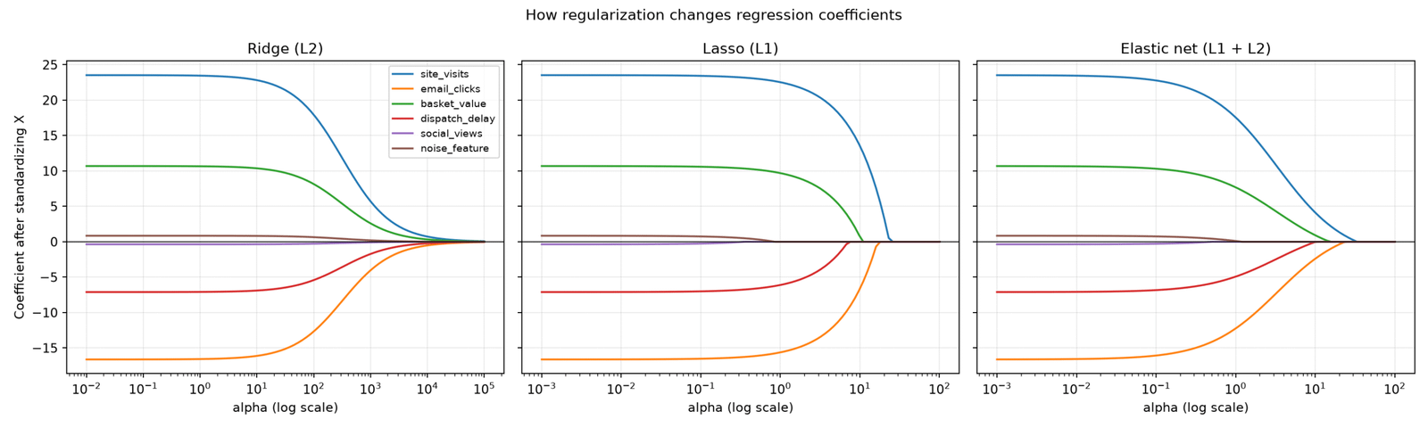
The result will be three coefficient-path plots.
Each colored line represents one feature’s coefficient. The horizontal axis shows alpha on a logarithmic scale; the vertical axis shows the fitted coefficient value.
We’ll deliberately create nearly orthogonal predictors for this first experiment. This makes the basic shrinking behavior especially clear, without the complications introduced by multicollinearity.
Step 1: Install the dependencies
You’ll need Python, NumPy, Matplotlib, and a current release of scikit-learn.
python -m venv .venv
Activate the virtual environment.
On macOS or Linux:
source .venv/bin/activate
On Windows PowerShell:
.venv\Scripts\Activate.ps1
Install the packages:
python -m pip install --upgrade numpy matplotlib scikit-learn
Step 2: Generate the coefficient-path plots
Save the following as coefficient_paths.py.
import matplotlib.pyplot as plt
import numpy as np

from sklearn.linear_model import ElasticNet, Lasso, Ridge
from sklearn.preprocessing import StandardScaler

rng = np.random.default_rng(7)

n = 320

feature_names = [
    "site_visits",
    "email_clicks",
    "basket_value",
    "dispatch_delay",
    "social_views",
    "noise_feature",
]

# Create approximately independent, orthogonal feature columns.
raw_random = rng.normal(size=(n, len(feature_names)))
raw_random -= raw_random.mean(axis=0)

q, _ = np.linalg.qr(raw_random)
z = q * np.sqrt(n)

# Give features dramatically different original scales.
raw_scales = np.array([5000, 200, 60, 3, 10000, 1])
X_raw = z * raw_scales

# This is a demonstration-only dataset, not a predictive
# evaluation. There is no test split in this experiment.
X = StandardScaler().fit_transform(X_raw)

# Four relevant features and two irrelevant ones.
true_coefs = np.array([24, -17, 11, -8, 0, 0])

y = (
    120
    + X @ true_coefs
    + rng.normal(0, 8, size=n)
)

# Ridge uses a different objective scaling from Lasso
# and ElasticNet, so its useful alpha range differs.
configurations = [
    (
        "Ridge (L2)",
        np.geomspace(1e-2, 1e5, 95),
        lambda a: Ridge(alpha=a),
    ),
    (
        "Lasso (L1)",
        np.geomspace(1e-3, 1e2, 95),
        lambda a: Lasso(
            alpha=a,
            max_iter=20000,
            tol=1e-7,
        ),
    ),
    (
        "Elastic net (L1 + L2)",
        np.geomspace(1e-3, 1e2, 95),
        lambda a: ElasticNet(
            alpha=a,
            l1_ratio=0.7,
            max_iter=20000,
            tol=1e-7,
        ),
    ),
]

fig, axes = plt.subplots(
    1, 3, figsize=(16, 4.8), sharey=True
)

for ax, (title, alphas, make_model) in zip(
    axes, configurations
):
    coefficient_paths = np.array([
        make_model(float(alpha)).fit(X, y).coef_
        for alpha in alphas
    ])

    for feature_index, name in enumerate(feature_names):
        ax.plot(
            alphas,
            coefficient_paths[:, feature_index],
            label=name,
        )

    ax.set_xscale("log")
    ax.axhline(0, color="black", linewidth=0.7)
    ax.set_title(title)
    ax.set_xlabel("alpha (log scale)")
    ax.grid(alpha=0.25)

    if title.startswith("Lasso"):
        for chosen_alpha in [0.1, 1.0, 10.0, 100.0]:
            idx = np.argmin(
                np.abs(alphas - chosen_alpha)
            )

            zeros = np.count_nonzero(
                coefficient_paths[idx] == 0
            )

            print(
                f"Lasso alpha ≈ {alphas[idx]:.3g}: "
                f"{zeros} exact zeros"
            )

axes[0].set_ylabel(
    "Coefficient after standardizing X"
)
axes[0].legend(fontsize=8, loc="upper right")

fig.suptitle(
    "How regularization changes regression coefficients"
)

fig.tight_layout()
fig.savefig("coefficient_paths.png", dpi=170)

plt.show()
Run it:
python coefficient_paths.py
The script saves coefficient_paths.png and displays the three plots.
Step 3: Read the ridge coefficient path
In the ridge subplot, each coefficient moves smoothly toward zero as alpha increases.
Because our demonstration features are orthogonal, each coefficient’s absolute magnitude decreases monotonically.
For orthogonal standardized features, ridge has a particularly simple relationship:
Ridge coefficient = OLS coefficient × n / (n + alpha)
This relationship explains why the plot looks so smooth.
Suppose an ordinary least-squares coefficient is 20, and we have 320 training observations.
At alpha = 320, its ridge estimate becomes approximately 10.
At alpha = 2,880, it becomes approximately 2.
The penalty progressively reduces its magnitude without abruptly removing it.
Even irrelevant features with small noisy coefficients generally remain nonzero.
That is important if your primary goal is better prediction rather than reducing the number of features.
Ridge says, in effect: keep the available information, but don’t allow the model to place too much trust in large coefficient estimates.
Step 4: Read the lasso coefficient path
The lasso plot behaves differently.
At very small alpha values, the coefficients are close to their ordinary least-squares estimates.
As alpha increases, some lines reach the horizontal zero axis and stay there.
For our seeded dataset, the script produces a progression similar to:
Lasso alpha ≈ 0.105: 0 exact zeros
Lasso alpha ≈ 0.952: 2 exact zeros
Lasso alpha ≈ 9.76: 3 exact zeros
Lasso alpha ≈ 100: 6 exact zeros
At moderate regularization, the two irrelevant features disappear.
At stronger regularization, even genuinely useful predictors begin disappearing because the penalty outweighs the reduction in training error they provide.
Eventually, all six coefficients become zero.
At that point, the model predicts the fitted intercept for every observation.
This illustrates an important concept:
More sparsity is not automatically better.
An overly large alpha can turn a useful predictive model into an underfitted constant predictor.
The objective is not to maximize the number of zero coefficients. It is to find a good balance between predictive performance and coefficient simplicity.
Step 5: Read the elastic net path
Elastic net’s path sits conceptually between the other two.
It has an L1 component, so coefficients can become exactly zero.
But it also has an L2 component, which modifies how surviving coefficients shrink and helps stabilize solutions when features are correlated.
We used an L1 mixing ratio of 0.7, meaning the model has a substantial sparsity-inducing component.
Try changing the value to 0.2 and rerunning the script. Then change it to 0.95.
Observe how the paths change.
A smaller mixing ratio generally produces behavior more reminiscent of ridge. A larger ratio approaches lasso.
The exact results depend on both the feature relationships and alpha, not simply the mixing ratio in isolation.
6. Cherry on the cake: lasso can arbitrarily choose between identical features
Here’s a surprising result with real practical consequences.
If two features contain exactly the same information, lasso can assign essentially the entire coefficient to one feature and zero to the other. Which one wins can depend on something as mundane as column order.
This isn’t evidence that the selected feature is more important.
It happens because the optimization problem has multiple equally good solutions.
Let’s demonstrate it.
Create two duplicate retail signals
Imagine an e-commerce analytics system has two columns:
-
Organic visits
-
Referral visits
Because of a logging mistake, both columns contain identical values.
We’ll fit lasso twice. The only difference between the runs is the order in which those columns are supplied.
We’ll also fit elastic net to the same data.
import numpy as np

from sklearn.linear_model import Lasso, ElasticNet
from sklearn.preprocessing import StandardScaler

rng = np.random.default_rng(4)

n = 250
signal = rng.normal(size=n)

# Two exactly identical predictors.
X = np.column_stack([signal, signal])

# A synthetic daily-orders target.
y = (
    40
    + 12 * signal
    + rng.normal(scale=2, size=n)
)

names = ["organic_visits", "referral_visits"]

for order in ([0, 1], [1, 0]):
    X_ordered = X[:, order]

    scaler = StandardScaler()
    X_scaled = scaler.fit_transform(X_ordered)

    lasso = Lasso(
        alpha=0.7,
        max_iter=50000,
        tol=1e-10,
        selection="cyclic",
    )

    elastic = ElasticNet(
        alpha=0.7,
        l1_ratio=0.5,
        max_iter=50000,
        tol=1e-10,
    )

    lasso.fit(X_scaled, y)
    elastic.fit(X_scaled, y)

    # Restore coefficients to the original column order.
    lasso_coefs = np.zeros(2)
    elastic_coefs = np.zeros(2)

    lasso_coefs[list(order)] = lasso.coef_
    elastic_coefs[list(order)] = elastic.coef_

    print(f"\nInput order: {[names[i] for i in order]}")

    for i, name in enumerate(names):
        print(
            f"{name:17s} "
            f"Lasso={lasso_coefs[i]:8.4f} "
            f"ElasticNet={elastic_coefs[i]:8.4f}"
        )
What happens?
With this seed, lasso places essentially the entire nonzero weight on whichever duplicated feature appears first.
Reversing the columns reverses the selected feature.
Elastic net instead distributes weight approximately equally across both features.
Why?
For identical predictors, many coefficient combinations produce exactly the same predictions.
Under an L1 penalty, two nonnegative coefficients that add up to the same number also have the same total absolute-value penalty.
For example, coefficients of 10 and 0 produce the same fitted contribution and the same L1 penalty as coefficients of 5 and 5 when the two feature columns are identical.
Lasso therefore has no unique reason to prefer one allocation.
The coordinate-descent optimizer must nevertheless return a particular solution. Its update order can determine the allocation.
Elastic net’s L2 component changes this.
For a fixed sum of two coefficients, splitting their values evenly minimizes the sum of their squares.
That favors sharing the coefficient weight instead of assigning all of it to one identical feature.
Why the issue extends beyond perfect duplicates
Real datasets rarely contain exact duplicates, but near-duplicates are extremely common.
Consider:
-
Website visits and page views
-
Advertising spend and advertising impressions
-
Property size in square feet and square meters
-
CPU utilization and processor busy time
-
Total order value and gross merchandise value
With strongly correlated predictors, small changes in the observations can alter which feature lasso retains.
A feature might survive regularization in one training sample and disappear in another.
That makes naive lasso-based feature selection unstable.
The current scikit-learn linear-model documentation explicitly notes the advantage of elastic net for correlated feature groups, and its sparse-signal example demonstrates the difficulty lasso has recovering the correct feature pattern when predictors are correlated.
A zero coefficient is not proof of irrelevance
This is the critical lesson.
If lasso sets an advertising-impressions coefficient to zero, it doesn’t necessarily mean impressions provide no information about orders.
It may mean the information is already represented by another correlated predictor.
Similarly, a surviving coefficient is not proof that a feature has an independently causal relationship with the target.
If interpretability or feature-selection stability matters, consider:
-
Examining feature correlations before modeling.
-
Repeating lasso selection across bootstrap or repeated training samples.
-
Measuring how frequently each feature survives.
-
Using elastic net when correlated groups should remain represented.
-
Grouping redundant features using domain knowledge.
-
Comparing feature groups rather than treating every selected coefficient as a discovery.
In other words, treat sparse coefficients as model outputs, not unquestionable scientific conclusions.
7. Choosing alpha with cross-validation
So far, we’ve manually swept alpha to learn how the models behave.
In a real predictive project, alpha should be chosen using training data rather than intuition alone.
Too little regularization can leave the model sensitive to noise.
Too much regularization can create substantial underfitting.
The correct amount depends on the dataset, target scale, feature relationships, and evaluation objective.
Scikit-learn provides three convenient estimators:
-
RidgeCVchooses ridge’s alpha. -
LassoCVchooses lasso’s alpha. -
ElasticNetCVchooses both alpha and, when given multiple candidates, the L1 mixing ratio.
Current scikit-learn supports explicit alpha arrays for these estimators. For elastic net, the l1_ratio parameter can also receive a list of candidate values.
How cross-validation works
Suppose we use five-fold cross-validation.
The training data is divided into five subsets.
For each candidate alpha:
-
Train on four subsets.
-
Evaluate on the remaining subset.
-
Repeat until every subset has served as validation data.
-
Average the validation errors.
-
Compare candidate alpha values.
The best candidate is selected according to the validation metric.
The model is then fitted again on the full training data with the selected settings.
This is better than choosing alpha according to training error because the validation folds simulate predictions on observations not used to fit the coefficients in that fold.
But cross-validation only works properly when the data-preparation workflow respects the validation boundaries.
An easy-to-miss preprocessing subtlety
There’s a distinction between placing an internally cross-validating estimator after a scaler and cross-validating an entire preprocessing pipeline.
For example, when a pipeline contains StandardScaler followed by LassoCV, the outer pipeline fits the scaler before LassoCV starts its own internal cross-validation.
The scaler has therefore seen all rows in that outer training set, including rows subsequently used as validation folds within LassoCV.
That can introduce a small amount of preprocessing leakage into the inner model-selection process.
It does not contaminate a completely separate test set, but it means the internal validation folds are not strictly isolated from the scaling operation.
For rigorous fold-local preprocessing, use GridSearchCV with a full pipeline containing both the scaler and model. The whole pipeline is refitted inside every cross-validation fold.
This distinction follows scikit-learn’s guidance on preventing leakage through cross-validated pipelines.
Let’s implement both approaches so you can see the difference in practice.
8. Complete experiment: built-in CV and leakage-safe model selection
We’ll now create a more realistic synthetic retail dataset.
Unlike the earlier coefficient-path experiment, these features are deliberately correlated.
Our dataset includes:
-
Website visits
-
Advertising impressions
-
Email clicks
-
Discount amount
-
Dispatch duration
-
One unrelated noise feature
We will keep 20% of the data completely separate as a test set.
The workflow will be:
-
Generate the dataset.
-
Split training and test data.
-
Demonstrate the three built-in CV estimators.
-
Use
GridSearchCVfor strict fold-local preprocessing. -
Compare model families using training cross-validation.
-
Evaluate the chosen model on the untouched test set.
Save the following as regularization_cv.py.
import numpy as np

from sklearn.linear_model import (
    ElasticNet,
    ElasticNetCV,
    Lasso,
    LassoCV,
    Ridge,
    RidgeCV,
)
from sklearn.metrics import mean_squared_error
from sklearn.model_selection import (
    GridSearchCV,
    KFold,
    train_test_split,
)
from sklearn.pipeline import Pipeline, make_pipeline
from sklearn.preprocessing import StandardScaler

rng = np.random.default_rng(12)

# --------------------------------------------------
# 1. Generate synthetic retail data
# --------------------------------------------------

n = 720

visits = rng.normal(12000, 2000, size=n)

impressions = (
    1.9 * visits
    + rng.normal(0, 600, size=n)
)

clicks = (
    0.075 * visits
    + rng.normal(0, 65, size=n)
)

discount = rng.uniform(0, 20, size=n)
dispatch_hours = rng.uniform(0, 7, size=n)
noise_column = rng.normal(size=n)

feature_names = [
    "visits",
    "impressions",
    "clicks",
    "discount",
    "dispatch_hours",
    "noise_column",
]

X = np.column_stack([
    visits,
    impressions,
    clicks,
    discount,
    dispatch_hours,
    noise_column,
])

# Visits, discount and dispatch time drive orders.
# Impressions and clicks largely duplicate visit information.
y = (
    40
    + 0.008 * visits
    + 2.2 * discount
    - 3.0 * dispatch_hours
    + rng.normal(0, 14, size=n)
)

# --------------------------------------------------
# 2. Keep the test set untouched
# --------------------------------------------------

X_train, X_test, y_train, y_test = train_test_split(
    X,
    y,
    test_size=0.2,
    random_state=42,
)

ridge_grid = np.geomspace(1e-2, 1e5, 40)
sparse_grid = np.geomspace(1e-3, 1e2, 36)

# --------------------------------------------------
# 3. Convenient built-in CV estimators
# --------------------------------------------------

built_in = {
    "RidgeCV": make_pipeline(
        StandardScaler(),
        RidgeCV(
            alphas=ridge_grid,
            cv=5,
            scoring="neg_mean_squared_error",
        ),
    ),
    "LassoCV": make_pipeline(
        StandardScaler(),
        LassoCV(
            alphas=sparse_grid,
            cv=5,
            max_iter=30000,
            tol=1e-6,
        ),
    ),
    "ElasticNetCV": make_pipeline(
        StandardScaler(),
        ElasticNetCV(
            alphas=sparse_grid,
            l1_ratio=[0.3, 0.6, 0.9, 1.0],
            cv=5,
            max_iter=30000,
            tol=1e-6,
        ),
    ),
}

print("Built-in cross-validation estimators")

for name, pipeline in built_in.items():
    pipeline.fit(X_train, y_train)

    chosen = pipeline[-1]

    extra = (
        f", l1_ratio={chosen.l1_ratio_:.2f}"
        if name == "ElasticNetCV"
        else ""
    )

    print(
        f"{name}: alpha={chosen.alpha_:.5g}{extra}"
    )

# --------------------------------------------------
# 4. Strict fold-local scaling with GridSearchCV
# --------------------------------------------------

folds = KFold(
    n_splits=5,
    shuffle=True,
    random_state=7,
)

configurations = {
    "Ridge": (
        Ridge(),
        {"model__alpha": ridge_grid},
    ),
    "Lasso": (
        Lasso(max_iter=30000, tol=1e-6),
        {"model__alpha": sparse_grid},
    ),
    "Elastic net": (
        ElasticNet(max_iter=30000, tol=1e-6),
        {
            "model__alpha": sparse_grid,
            "model__l1_ratio": [0.3, 0.6, 0.9, 1.0],
        },
    ),
}

searches = {}

for name, (estimator, params) in configurations.items():
    pipeline = Pipeline([
        ("scale", StandardScaler()),
        ("model", estimator),
    ])

    search = GridSearchCV(
        pipeline,
        param_grid=params,
        cv=folds,
        scoring="neg_mean_squared_error",
        n_jobs=1,
        refit=True,
    )

    search.fit(X_train, y_train)
    searches[name] = search

    cv_rmse = np.sqrt(-search.best_score_)

    print(
        f"{name}: CV RMSE={cv_rmse:.3f}; "
        f"best={search.best_params_}"
    )

# --------------------------------------------------
# 5. Select using TRAINING CV, not test performance
# --------------------------------------------------

best_name = max(
    searches,
    key=lambda name: searches[name].best_score_,
)

best_pipeline = searches[best_name].best_estimator_

test_rmse = np.sqrt(
    mean_squared_error(
        y_test,
        best_pipeline.predict(X_test),
    )
)

print(
    f"Selected: {best_name}; "
    f"untouched-test RMSE={test_rmse:.3f}"
)

# --------------------------------------------------
# 6. Inspect the selected model's coefficients
# --------------------------------------------------

for name, value in zip(
    feature_names,
    best_pipeline[-1].coef_,
):
    print(
        f"{name:16s}: {value:+.3f} "
        "(per training standard deviation)"
    )
Run it:
python regularization_cv.py
Understanding the output
Our run (scikit-learn 1.9.1, NumPy 2.5.4) printed:
Built-in cross-validation estimators
RidgeCV: alpha=0.94267
LassoCV: alpha=0.19307
ElasticNetCV: alpha=0.19307, l1_ratio=1.00
Ridge: CV RMSE=13.627
Lasso: CV RMSE=13.611
Elastic net: CV RMSE=13.611 (l1_ratio=1.0)
Selected: Lasso; untouched-test RMSE=13.989
visits          : +15.138 (per training standard deviation)
impressions     : +0.000 (per training standard deviation)
clicks          : +0.856 (per training standard deviation)
discount        : +11.972 (per training standard deviation)
dispatch_hours  : -6.914 (per training standard deviation)
noise_column    : -0.752 (per training standard deviation)
The best={...} dictionaries the script also prints are shortened here.
With the stated random seed, the strict pipeline search produces cross-validation RMSE values around 13.6 orders for the candidate families.
Lasso and elastic net with an L1 mixing ratio of 1 can achieve essentially the same performance, because an elastic net with l1_ratio=1 has the lasso objective.
In this example, the chosen model’s untouched-test RMSE is approximately 14 orders.
The precise selected configuration can depend on numerical details and ties, so the meaningful result is the workflow rather than any particular winning alpha.
The printed coefficients show the contributions of the predictors after standardization.
For example, website visits can receive a substantial positive coefficient while advertising impressions receive zero.
That’s not evidence that advertising impressions have no predictive relationship with orders.
We intentionally generated impressions as a noisy multiple of visits. The model can already obtain much of that information from website visits.
The fitted coefficient allocation reflects this redundancy.
Why use RMSE?
Root mean squared error measures prediction error in the original target’s units.
Here, the units are daily orders.
It is calculated as:
RMSE = √(mean of squared prediction errors)
An RMSE of 14 means the square root of the average squared error is 14 orders. It is not the same as saying predictions are always within 14 orders.
RMSE penalizes larger mistakes more heavily than smaller mistakes, making it a reasonable metric for many regression tasks.
In scikit-learn, scoring values are conventionally maximized.
Consequently, neg_mean_squared_error returns negative MSE scores so that better models have higher values.
That’s why the code takes the negative of the best cross-validation score before calculating its square root.
Why the test set must remain untouched
The final test set exists to estimate how the selected workflow performs on new observations.
It should not be used to:
-
Choose alpha.
-
Decide between ridge and lasso.
-
Select a different mixing ratio.
-
Change preprocessing based on test performance.
-
Repeatedly revise features until the score improves.
Our code selects the winning model family using training cross-validation only.
Then it evaluates that selection once on the held-out test data.
If you compare many different modeling strategies across multiple experiments and want an unbiased performance estimate for the entire selection process, use nested cross-validation or reserve a truly final evaluation dataset.
Also remember that ordinary shuffled folds assume observations are reasonably exchangeable.
For time-ordered retail activity, use time-aware validation so future observations cannot influence predictions of earlier ones. For repeated stores, customers, or devices, group-aware splitting may be necessary.
9. How to interpret coefficients after regularization
Regularization changes what a coefficient means operationally.
A standardized regression coefficient still describes the change in the prediction associated with a one-standard-deviation increase in its feature, holding the other model inputs constant.
But that number is now intentionally biased toward zero.
The coefficient is a compromise between explaining the data and satisfying the regularization penalty.
That leads to several consequences.
Smaller coefficients aren’t necessarily weaker causal effects
Suppose ridge estimates a standardized discount coefficient of 8 while ordinary regression estimates 11.
The difference does not demonstrate that the real-world influence of discounts has declined.
Ridge has deliberately introduced shrinkage.
Likewise, the relative sizes of penalized coefficients do not automatically rank the independent causal importance of features, especially when predictors are correlated.
Zero is a model-selection outcome
For lasso and elastic net, exact zeros are meaningful properties of the fitted model.
They identify features whose coefficients the optimizer eliminated at a particular penalty strength.
But feature selection is conditional on:
-
Which predictors were supplied.
-
How they were scaled.
-
Which observations were used.
-
The chosen alpha.
-
The correlation structure.
-
The optimizer’s numerical behavior.
If any of those change, the selected feature subset may change.
Coefficients aren’t always directly comparable across datasets
Even after scaling, a coefficient is measured per standard deviation of its feature.
If two datasets have different feature distributions, the numerical value of one standardized coefficient can change partly because the underlying standard deviation changed.
To convert standardized coefficients back to original feature units, divide each standardized coefficient by the corresponding training standard deviation.
For a model with an intercept, the original-scale intercept must also be adjusted to account for feature means.
This is especially relevant when delivering coefficients to stakeholders who expect interpretations in dollars, hours, visits, or other real-world units.
10. Common mistakes to avoid
Regularization is simple conceptually, but several mistakes can undermine an otherwise reasonable experiment.
Mistake 1: Applying regularization without scaling
When different features have radically different units, the penalty treats them unequally.
Fix: Use training-fitted scaling, preferably in a pipeline that participates in cross-validation.
Mistake 2: Treating alpha values as comparable across models
Ridge and lasso have different objective scaling conventions.
An alpha of 1 in ridge is not equivalent to an alpha of 1 in lasso.
Fix: Tune separate, appropriate alpha ranges for each model family.
Mistake 3: Selecting alpha using the test set
Choosing the alpha that yields the smallest test error turns the test set into a validation set.
Fix: Choose hyperparameters through training cross-validation, then evaluate on the test set.
Mistake 4: Assuming lasso always discovers the correct features
Strong correlation can make feature selection unstable.
Fix: Inspect correlations, test selection stability, and consider elastic net or domain-informed grouping.
Mistake 5: Using extremely small positive alpha as though optimization is free
When alpha approaches zero, the model approaches an unregularized solution. With highly collinear data, this can make numerical optimization harder, particularly for coordinate-descent methods.
Fix: Choose a sensible positive grid, monitor convergence warnings, and compare against ordinary least squares where appropriate.
For unregularized fitting, use LinearRegression rather than forcing Lasso(alpha=0). Scikit-learn explicitly recommends this for numerical reasons.
Mistake 6: Ignoring convergence warnings
Lasso and elastic net use iterative optimization methods.
If the optimizer stops before convergence, the reported coefficient values may be inaccurate.
Fix: Standardize features, increase max_iter when necessary, and check solver tolerance and convergence diagnostics.
Mistake 7: Maximizing sparsity instead of predictive quality
A model with just two predictors is not automatically better than one with twenty.
Fix: Evaluate prediction errors and model stability. Prefer additional sparsity only when the associated trade-off is worthwhile for your application.
11. Ridge vs. lasso vs. elastic net: which should you choose?
The best regularizer depends on the structure of your data and what you want the model to accomplish.
| Situation | Good starting point | Why |
|---|---|---|
| Many correlated predictors | Ridge | Stabilizes coefficients while retaining predictors |
| Most features may contribute | Ridge | Shrinkage without aggressive feature elimination |
| Only a few features expected to matter | Lasso | Can produce a sparse coefficient vector |
| Need a compact predictive model | Lasso or elastic net | Can eliminate some inputs |
| Strongly correlated groups, with desired sparsity | Elastic net | Combines feature elimination with more stable group behavior |
| Unsure about feature structure | Compare all three | Use consistent validation and metrics |
These are starting points, not rules guaranteeing the best prediction score.
In practice, a cross-validated ridge model can beat a sparse model on one dataset, while elastic net or lasso can outperform it on another.
One helpful mental model is:
-
Ridge: I believe many features have useful information, but their coefficients need restraint.
-
Lasso: I believe a relatively small subset of features can explain most of the target.
-
Elastic net: I want sparsity, but I don’t trust the model to make stable choices among correlated features.
And if interpretability matters more than shaving a small amount off prediction error, you may prefer a simpler or more stable model even when its validation performance is marginally worse.
That is a modeling decision, not a limitation of cross-validation.
12. A practical checklist for production projects
Before shipping a regularized linear regression model, review the following:
- Split training, validation, and testing appropriately for the data.
- Examine missing values, outliers, feature scales, and strong correlations.
- Standardize numeric predictors within the training pipeline.
- Compare an unregularized baseline and relevant regularized models.
- Tune alpha using cross-validation without preprocessing leakage.
- Tune
l1_ratiowhen considering elastic net. - Examine coefficient paths rather than trusting one alpha blindly.
- Investigate whether feature selection changes across resamples.
- Compare against a simple baseline such as predicting the training-set mean.
- Evaluate the selected workflow on untouched data.
- Preserve the fitted preprocessing and model together for inference.
- Monitor prediction quality and data distribution changes after deployment.
For larger feature sets, exhaustive grid search can be expensive, particularly when tuning both alpha and mixing ratios. The built-in CV estimators can be computationally attractive because their algorithms exploit regularization paths. The appropriate choice depends on whether you need strict fold-local preprocessing and how complex your preprocessing pipeline is.
13. Final takeaways
Ridge, lasso, and elastic net are not merely three interchangeable ways of making linear regression less likely to overfit.
Their penalties shape the fitted coefficients differently.
Ridge uses L2 regularization to discourage large coefficients through a squared penalty. Its coefficient paths are smooth, and it generally retains predictors with reduced weights.
Lasso uses L1 regularization to create sparsity. Its constraint geometry has corners aligned with coordinate axes, making exactly zero coefficients natural solutions.
Elastic net combines L1 and L2 to provide a compromise between sparsity and stability, especially when several predictors carry overlapping information.
But the most important operational lessons extend beyond the penalties themselves.
Standardization is essential for meaningful regularization. Alpha must be chosen through a defensible validation procedure. And zero coefficients must not be interpreted as definitive evidence that a feature contains no useful information.
The experiment with duplicate features makes that last lesson concrete: lasso can assign all the weight to one of two identical predictors simply because of the way the optimization problem is resolved.
A sparse model is not necessarily a reliable explanation of the data-generating process.
Your next experiment
Take a neutral regression dataset—housing prices, retail demand, energy consumption, or server latency—and apply the complete workflow:
-
Plot coefficient paths for ridge, lasso, and elastic net.
-
Tune their regularization strengths using fold-local preprocessing and cross-validation.
-
Compare prediction quality and the number of nonzero coefficients.
-
Introduce a highly correlated copy of an existing feature and repeat the experiment.
-
Check whether the selected features and coefficient values remain stable.
Don’t stop at reporting the lowest RMSE. Examine what happens to the coefficients, why it happens, and whether those changes make your model more useful.
That’s when regularization becomes more than a hyperparameter—and starts becoming a tool you genuinely understand.