
LEARN · MATHEMATICS FOR MACHINE LEARNING
Imagine four hikers trying to reach the bottom of the same mountain valley. Each can measure the slope beneath their feet, but none has a complete map of the terrain.
One always steps directly downhill. Another builds momentum. A third adjusts its stride depending on how steep the terrain has been. The fourth combines momentum with adaptive step sizes.
These hikers represent four optimization algorithms:
-
Gradient descent (SGD): Follows the negative gradient using a fixed learning rate.
-
Momentum: Accumulates gradients to maintain movement in consistent directions.
-
RMSProp: Adjusts each parameter’s step size using a running average of squared gradients.
-
Adam: Combines moving averages of gradients and squared gradients, with bias correction.
All four optimize the same mathematical objective, but their trajectories can look dramatically different.
A narrow valley may cause ordinary gradient descent to zigzag. Momentum can accelerate movement along the valley. RMSProp can reduce sensitivity to steep directions. Adam can combine these benefits, although it is not guaranteed to win.
In this tutorial, we’ll implement all four algorithms from scratch using NumPy, race them across a nonlinear loss surface, and animate their trajectories with Matplotlib.
We’ll also investigate a surprising counterexample: a smooth loss surface where ordinary SGD reaches an excellent solution while Adam moves away from the optimum and struggles to recover.
By the end, you’ll understand not only how these optimizers work, but also why their behavior depends on the geometry of the objective function.
1. Understanding the optimization problem
An optimizer attempts to find parameters that minimize a loss function.
For a two-dimensional objective, we can write:
Loss = L(x, y)
Here, x and y are parameters that the algorithm can adjust.
The gradient measures how rapidly the loss changes in each coordinate:
Gradient = ∇L(x, y) = (∂L/∂x, ∂L/∂y)
The gradient points in the direction of steepest local increase. To minimize the loss, a basic optimizer moves in the opposite direction.
For ordinary gradient descent, the update is:
θ_new = θ_old − η · ∇L(θ_old)
Where:
-
θ represents the vector of parameters.
-
η is the learning rate.
-
∇L is the gradient at the current position.
The learning rate controls the step size. Too small, and optimization can progress painfully slowly. Too large, and the algorithm may overshoot the minimum or even diverge.
Why loss-surface geometry matters
Consider three different shapes.
A circular bowl: Both coordinates have similar curvature. Ordinary gradient descent usually works well with a suitable learning rate.
A narrow elliptical valley: One direction is much steeper than the other. Gradient descent may bounce between the valley walls while making slow progress toward the minimum.
A curved valley: The direction toward the minimum changes as optimization proceeds. Momentum can help, but excessive momentum can also send the optimizer across the valley or past a turn.
Real machine-learning loss landscapes can be much more complicated than these examples. They may involve millions or billions of parameters, flat regions, saddles, and complicated interactions between directions.
Our two-dimensional experiment deliberately simplifies the problem so that we can watch every update.
2. Meet the four optimizers
Before implementing the race, let’s examine the update rules.
2.1 Plain gradient descent: the baseline
For a parameter vector θ, standard gradient descent uses:
θ_t = θ_(t−1) − η · g_t
Here, g_t is the gradient at iteration t.
This method has almost no memory. Each step depends only on the current gradient.
Its advantages are simplicity, predictable behavior under suitable smoothness and learning-rate conditions, and minimal optimizer state.
Its disadvantages become visible on poorly conditioned surfaces. The algorithm must often use a small learning rate to avoid instability along the steepest direction, which makes movement along flatter directions slow.
A terminology detail matters: our experiment uses the exact gradient of a deterministic function. Technically, it is full-gradient descent, not stochastic gradient descent. We’ll label it SGD in the visualization because that is a familiar baseline name, but no minibatch sampling or gradient noise is involved.
2.2 Momentum: remembering previous directions
Momentum maintains a velocity vector that accumulates gradients:
v_t = μ · v_(t−1) + g_t
θ_t = θ_(t−1) − η · v_t
Here, μ is the momentum coefficient. We’ll use 0.9.
When successive gradients point in roughly the same direction, the velocity grows. When gradients repeatedly change sign, their contributions can cancel.
This is particularly useful in narrow valleys:
-
Across the valley, oscillating gradient components partially cancel.
-
Along the valley, consistently directed gradients accumulate.
-
The optimizer can travel farther per update in the persistent direction.
The trade-off is inertia. Momentum may overshoot a minimum or take several iterations to recover after the valley changes direction.
Our implementation uses classical, unnormalized momentum rather than Nesterov momentum. The difference matters when reproducing experiments or comparing framework configurations.
2.3 RMSProp: adapting to gradient magnitude
RMSProp tracks an exponentially weighted average of squared gradients.
For every parameter coordinate:
s_t = ρ · s_(t−1) + (1 − ρ) · g_t²
θ_t = θ_(t−1) − η · g_t / (√s_t + ε)
The operations on vectors are performed coordinate by coordinate.
The parameter ρ controls the decay of the squared-gradient history. The small positive ε prevents division by zero and improves numerical stability.
The intuition is straightforward:
-
A coordinate with consistently large gradients builds a larger squared-gradient average.
-
Its effective step size becomes smaller.
-
A coordinate with smaller gradients can receive a relatively larger step.
This can improve progress on surfaces where different coordinates have vastly different curvature or gradient scales.
RMSProp does not automatically guarantee a decreasing loss at every iteration. Its adaptive scaling can still cause oscillations or overshooting, especially near a narrow optimum.
2.4 Adam: momentum plus adaptive scaling
Adam combines two exponential moving averages.
The first tracks the gradient:
m_t = β₁ · m_(t−1) + (1 − β₁) · g_t
The second tracks the squared gradient:
v_t = β₂ · v_(t−1) + (1 − β₂) · g_t²
Because both averages start at zero, Adam applies bias correction:
m̂_t = m_t / (1 − β₁ᵗ)
v̂_t = v_t / (1 − β₂ᵗ)
Finally, Adam updates the parameters:
θ_t = θ_(t−1) − η · m̂_t / (√v̂_t + ε)
We’ll use β₁ = 0.9, β₂ = 0.999, and ε = 1e−8.
These are also the familiar default beta and epsilon settings documented for the current PyTorch Adam implementation.
Adam combines directional memory with coordinate-wise scaling. That makes it a useful general-purpose optimizer, especially when gradients vary substantially across parameters.
However, its adaptive normalization means that the magnitude of a parameter update is not necessarily proportional to the magnitude of its gradient.
That observation will become central to our counterexample.
3. Choosing a challenging loss surface
For our first experiment, we’ll use the Rosenbrock function, a classic nonlinear optimization benchmark.
Its two-dimensional form is:
L(x, y) = (1 − x)² + 100(y − x²)²
The global minimum is located at:
(x, y) = (1, 1), with L = 0
The first term pulls x toward 1. The second term penalizes deviations from the curved valley defined by y = x².
The result is a banana-shaped valley.
This objective is especially useful for visualization because it combines:
-
A steep direction across the valley.
-
A relatively flat direction along the valley.
-
Curvature that changes as parameters move.
-
A known global minimum for evaluating results.
Although the function is nonconvex, it has a single local minimum, which is also global. This makes it a clean demonstration of geometric optimization challenges without introducing competing local minima.
Computing the exact gradient
We can differentiate the objective analytically.
∂L/∂x = −2(1 − x) − 400x(y − x²)
∂L/∂y = 200(y − x²)
These derivatives let us evaluate the precise gradient at any coordinate, without numerical differentiation or a machine-learning framework.
We’ll initialize all four algorithms at:
Start = (−1.5, 1.5)
At this position, the loss is 62.5.
Each optimizer will perform 400 parameter updates. They will all see exactly the same objective and start from exactly the same point.
That means differences in their trajectories come from the update algorithms and the hyperparameters we choose, rather than different training data or random initialization.
4. Preparing the Python environment
Our experiment requires only three external Python libraries.
-
NumPy: Parameter vectors, numerical operations, and loss calculations.
-
Matplotlib: Contour plots, trajectory plots, and animations.
-
Pillow: Writing animated GIF files.
We don’t need TensorFlow, PyTorch, scikit-learn, datasets, or a GPU.
Use a modern Python environment, ideally Python 3.11 or newer.
Create a virtual environment and install the dependencies:
python -m venv .venv
source .venv/bin/activate
python -m pip install --upgrade pip
python -m pip install "numpy>=2.0" "matplotlib>=3.10" "pillow>=11"
These commands target bash-compatible shells on Linux and macOS. On Windows, the environment activation command differs.
We’ll use Matplotlib’s current FuncAnimation API to update existing plot artists, and PillowWriter to save the animation as a GIF. These interfaces are supported in the current Matplotlib documentation.
The implementation will generate three files:
| Output file | Purpose |
|---|---|
| optimizer_race.gif | Animated race across the Rosenbrock surface |
| optimizer_final.png | Final trajectories and loss curves |
| adam_counterexample.png | The pathological comparison between SGD and Adam |
The animation updates the trajectories from precomputed optimization histories. This is intentional: rendering a frame must not change an optimizer’s internal state, because an animation callback may be invoked more than once.
That separation makes the experiment deterministic, easier to debug, and safe to export.
5. Implementing the complete optimizer race
Create a file named optimizer_race.py and add the following implementation.
The script contains both experiments. First, it animates four optimizers on the Rosenbrock surface. Then, it constructs our pathological surface and compares SGD with Adam.
Everything is self-contained, including the gradient calculations, optimizer state, plotting, and GIF generation.
import numpy as np
import matplotlib

matplotlib.use("Agg")

import matplotlib.pyplot as plt
from matplotlib.animation import FuncAnimation, PillowWriter
from matplotlib.colors import LogNorm


# --------------------------------------------------
# Experiment 1: Rosenbrock loss surface
# --------------------------------------------------

def rosenbrock(x, y):
    return (1.0 - x) ** 2 + 100.0 * (y - x ** 2) ** 2


def rosenbrock_gradient(position):
    x, y = position
    return np.array([
        -2.0 * (1.0 - x) - 400.0 * x * (y - x ** 2),
        200.0 * (y - x ** 2),
    ])


# --------------------------------------------------
# Four optimizers implemented from scratch
# --------------------------------------------------

def optimize(gradient_fn, start, method, learning_rate, steps):
    position = np.asarray(start, dtype=float).copy()

    first = np.zeros_like(position)
    second = np.zeros_like(position)

    trajectory = np.empty((steps + 1, position.size))
    trajectory[0] = position

    for step in range(1, steps + 1):
        gradient = gradient_fn(position)

        if method == "SGD":
            direction = gradient

        elif method == "Momentum":
            first = 0.9 * first + gradient
            direction = first

        elif method == "RMSProp":
            second = 0.9 * second + 0.1 * gradient ** 2
            direction = gradient / (np.sqrt(second) + 1e-8)

        elif method == "Adam":
            first = 0.9 * first + 0.1 * gradient
            second = 0.999 * second + 0.001 * gradient ** 2

            corrected_first = first / (1.0 - 0.9 ** step)
            corrected_second = second / (1.0 - 0.999 ** step)

            direction = corrected_first / (
                np.sqrt(corrected_second) + 1e-8
            )

        else:
            raise ValueError(f"Unknown optimizer: {method}")

        position -= learning_rate * direction

        if not np.all(np.isfinite(position)):
            raise FloatingPointError(
                f"{method} diverged at iteration {step}"
            )

        trajectory[step] = position

    return trajectory


# --------------------------------------------------
# Animate the four-optimizer race
# --------------------------------------------------

def make_race():
    steps = 400
    start = np.array([-1.5, 1.5])

    learning_rates = {
        "SGD": 0.0025,
        "Momentum": 0.001,
        "RMSProp": 0.02,
        "Adam": 0.3,
    }

    trajectories = {
        name: optimize(
            rosenbrock_gradient, start, name, lr, steps
        )
        for name, lr in learning_rates.items()
    }

    losses = {
        name: rosenbrock(path[:, 0], path[:, 1])
        for name, path in trajectories.items()
    }

    # Create the contour grid.
    xs = np.linspace(-2.05, 2.05, 260)
    ys = np.linspace(-0.4, 3.0, 260)
    xx, yy = np.meshgrid(xs, ys)
    zz = rosenbrock(xx, yy)

    fig, (ax_surface, ax_loss) = plt.subplots(
        1, 2, figsize=(12, 5)
    )

    filled = ax_surface.contourf(
        xx,
        yy,
        zz,
        levels=np.geomspace(1e-3, 1e4, 32),
        norm=LogNorm(vmin=1e-3, vmax=1e4),
        cmap="viridis",
        extend="both",
    )

    fig.colorbar(
        filled,
        ax=ax_surface,
        label="Loss (log color scale)",
    )

    ax_surface.scatter(
        *start,
        s=70,
        facecolors="white",
        edgecolors="black",
        zorder=10,
        label="Start",
    )

    ax_surface.scatter(
        1.0,
        1.0,
        marker="*",
        s=180,
        color="yellow",
        edgecolors="black",
        zorder=10,
        label="Global minimum",
    )

    ax_surface.set(
        xlim=(-2.05, 2.05),
        ylim=(-0.4, 3.0),
        xlabel="x",
        ylabel="y",
        title="Paths on the Rosenbrock surface",
    )
    ax_surface.set_aspect("equal", adjustable="box")

    ax_loss.set(
        xlim=(0, steps),
        ylim=(1e-4, 1e3),
        xlabel="Optimizer step",
        ylabel="Loss",
        title="Loss versus iteration",
    )

    ax_loss.set_yscale("log")
    ax_loss.grid(True, which="both", alpha=0.2)

    # Create reusable artists.
    artists = {}

    for name in learning_rates:
        trail, = ax_surface.plot(
            [], [], linewidth=2, label=name
        )

        dot, = ax_surface.plot(
            [],
            [],
            marker="o",
            markersize=6,
            color=trail.get_color(),
        )

        curve, = ax_loss.plot(
            [],
            [],
            linewidth=2,
            label=name,
            color=trail.get_color(),
        )

        artists[name] = (trail, dot, curve)

    ax_surface.legend(loc="upper right", fontsize=8)
    ax_loss.legend(loc="upper right")
    fig.tight_layout()

    def update(step):
        changed = []

        for name, path in trajectories.items():
            trail, dot, curve = artists[name]

            trail.set_data(
                path[:step + 1, 0],
                path[:step + 1, 1],
            )

            dot.set_data(
                path[step:step + 1, 0],
                path[step:step + 1, 1],
            )

            curve.set_data(
                np.arange(step + 1),
                losses[name][:step + 1],
            )

            changed.extend((trail, dot, curve))

        ax_loss.set_title(
            f"Loss versus iteration (step {step})"
        )

        return changed

    animation = FuncAnimation(
        fig,
        update,
        frames=range(0, steps + 1, 10),
        interval=80,
        blit=False,
        repeat=False,
    )

    animation.save(
        "optimizer_race.gif",
        writer=PillowWriter(fps=12),
        dpi=75,
    )

    # Save the final frame separately.
    update(steps)
    fig.savefig("optimizer_final.png", dpi=150)
    plt.close(fig)

    print("Rosenbrock final losses after 400 steps:")

    for name, values in losses.items():
        print(f"  {name:8s}: {values[-1]:.6f}")


# --------------------------------------------------
# Experiment 2: The pathological plateau
# --------------------------------------------------

def plateau_loss(points):
    squared_radius = np.sum(
        np.asarray(points) ** 2,
        axis=-1,
    )
    return 2.0 * squared_radius / (
        1.0 + 100.0 * squared_radius
    )


def plateau_gradient(position):
    squared_radius = float(
        np.dot(position, position)
    )
    return 4.0 * position / (
        1.0 + 100.0 * squared_radius
    ) ** 2


def make_counterexample():
    steps = 80
    start = np.array([0.03, -0.04])

    paths = {
        name: optimize(
            plateau_gradient,
            start,
            name,
            0.2,
            steps,
        )
        for name in ("SGD", "Adam")
    }

    histories = {
        name: plateau_loss(path)
        for name, path in paths.items()
    }

    fig, (ax_path, ax_loss) = plt.subplots(
        1, 2, figsize=(11, 4.5),
        constrained_layout=True,
    )

    axis = np.linspace(-1.0, 1.0, 280)
    xx, yy = np.meshgrid(axis, axis)

    surface_points = np.stack(
        (xx, yy),
        axis=-1,
    )

    image = ax_path.contourf(
        xx,
        yy,
        plateau_loss(surface_points),
        levels=np.linspace(0.0, 0.0199, 26),
        cmap="magma",
        extend="max",
    )

    fig.colorbar(image, ax=ax_path, label="Loss")

    ax_path.plot(
        0.0, 0.0, "*",
        color="white",
        markersize=14,
        markeredgecolor="black",
        label="Minimum",
    )

    ax_path.plot(
        *start,
        marker="o",
        color="cyan",
        linestyle="None",
        label="Start",
    )

    for name, path in paths.items():
        ax_path.plot(
            path[:, 0],
            path[:, 1],
            linewidth=2,
            label=name,
        )

    ax_path.set(
        xlim=(-1, 1),
        ylim=(-1, 1),
        xlabel="x",
        ylabel="y",
        title="A small basin and a flat plateau",
    )

    ax_path.set_aspect("equal", adjustable="box")
    ax_path.legend(loc="lower right")

    for name, history in histories.items():
        ax_loss.semilogy(
            np.maximum(history, 1e-12),
            label=name,
            linewidth=2,
        )

    ax_loss.set(
        xlabel="Optimizer step",
        ylabel="Loss (clipped at 1e-12)",
        title="Same starting point and learning rate",
    )

    ax_loss.grid(True, which="both", alpha=0.2)
    ax_loss.legend()

    fig.savefig("adam_counterexample.png", dpi=150)
    plt.close(fig)

    print("Plateau losses (same learning rate, 0.2):")

    for name, history in histories.items():
        print(
            f"  {name:8s}: start={history[0]:.6f}, "
            f"step 1={history[1]:.6f}, "
            f"step 80={history[-1]:.6e}"
        )


if __name__ == "__main__":
    make_race()
    make_counterexample()
Run the script from your terminal:
python optimizer_race.py
The script uses a noninteractive plotting backend, so it works in headless environments as well as desktop Python installations. It saves files instead of requiring a graphical window.
Depending on your machine, GIF generation may take several seconds or longer because Matplotlib must render each frame.
6. Watching the optimizers race
The first output contains two synchronized views.
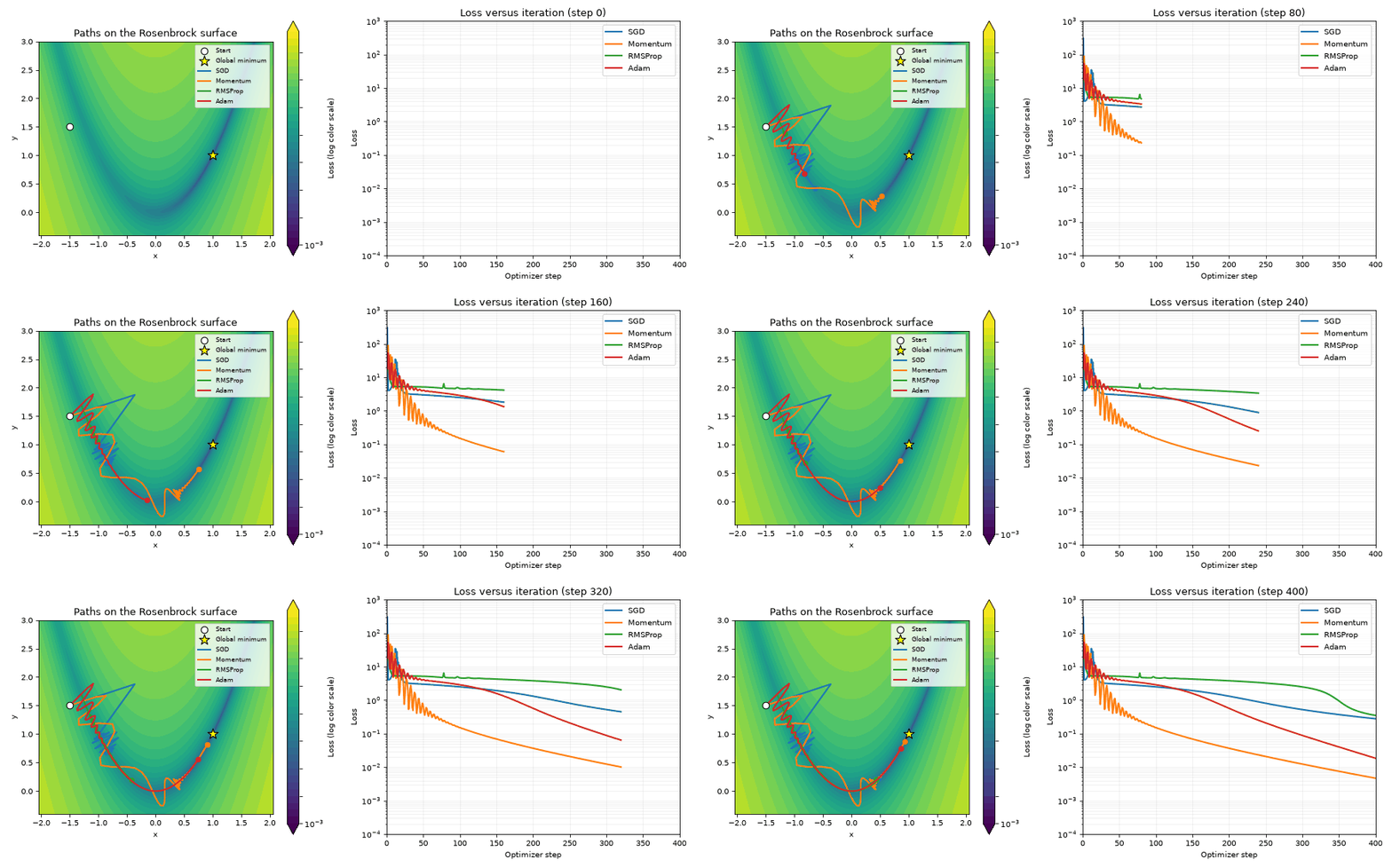
On the left, a contour plot shows the Rosenbrock surface. Darker areas represent lower losses, and the star indicates the global minimum.
On the right, a logarithmic plot shows the loss after each optimizer update.
This pairing is important. A trajectory can look geometrically impressive without producing a particularly low loss. Conversely, an optimizer may make substantial progress in objective value while appearing to travel only a short distance.
The logarithmic vertical axis makes improvements across several orders of magnitude visible.
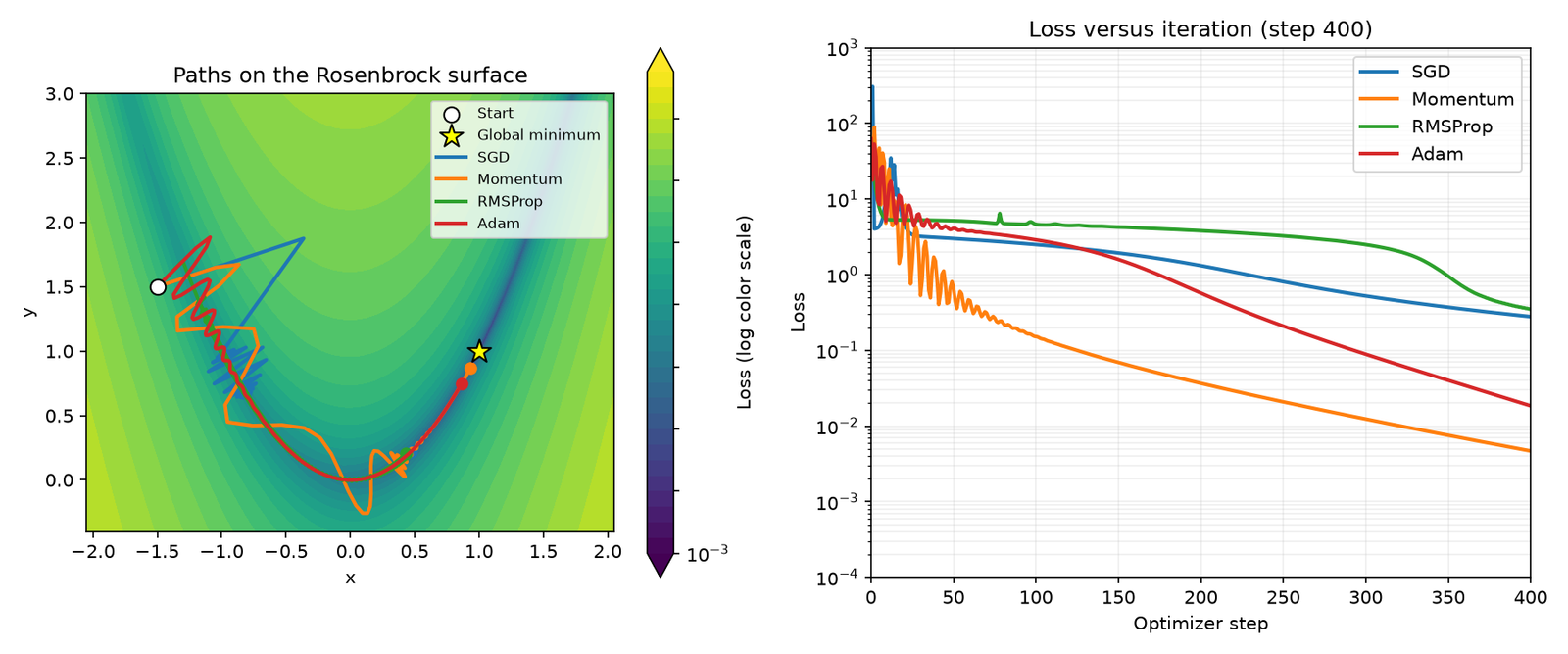
Results after 400 steps
Running the experiment with the supplied hyperparameters produces these approximate final losses:
| Optimizer | Learning rate | Final loss |
|---|---|---|
| SGD | 0.0025 | 0.279071 |
| Momentum | 0.001 | 0.004679 |
| RMSProp | 0.02 | 0.350917 |
| Adam | 0.3 | 0.018464 |
In this particular race, momentum produces the smallest final loss.
Adam finishes second. Ordinary gradient descent improves steadily but remains farther from the optimum. RMSProp eventually makes progress along the curved valley but does not reach the same low-loss region within the allotted steps.
These values come from the deterministic implementation above, rather than a general benchmark across optimization problems.
Why do the trajectories look different?
SGD initially makes a large jump. Its first gradient contains a substantial component along x. Because ordinary gradient descent directly multiplies this gradient by the learning rate, the first update can move it across the valley.
The loss initially increases before the optimizer recovers.
This is a useful reminder that even a differentiable, nonnegative objective does not guarantee monotonically decreasing loss under an arbitrary fixed learning rate.
Momentum oscillates but accelerates through the valley. Early updates swing across the curved region. As the direction of improvement becomes more persistent, accumulated velocity helps it make faster progress.
The initial oscillations are not evidence that optimization has failed. They reflect inertia interacting with the steep sides of the valley.
RMSProp changes its coordinate-wise scaling continuously. This helps control the effect of large gradient components, but it does not necessarily align updates with the valley’s curved geometry.
It can spend many iterations making comparatively slow progress.
Adam takes a different route. Its first-moment memory and second-moment normalization produce a distinct trajectory. With the relatively large learning rate chosen for this synthetic function, it eventually approaches the minimum quite closely.
However, it still trails the tuned momentum configuration after 400 updates.
A crucial fairness warning
The learning rates differ deliberately.
Using the same numerical learning rate for all four methods would not necessarily be fair because the methods scale their gradients differently.
For example, a learning rate of 0.3 in Adam does not mean its updates are directly comparable in magnitude to those of ordinary gradient descent at a learning rate of 0.3.
The purpose of this experiment is to reveal optimization dynamics, not to declare a universal winner.
To compare algorithms rigorously, we would need to tune each optimizer over a reasonable hyperparameter range, use a consistent evaluation budget, and repeat experiments across different objectives and initializations.
For deterministic two-dimensional functions, we can count gradient evaluations directly. In larger machine-learning systems, we should also measure wall-clock time, memory consumption, and validation performance.
7. How the animation works internally
The animation pipeline follows three stages.
Stage 1: Precompute the trajectories
Before rendering anything, we execute all optimizer updates and store the resulting parameter positions.
A trajectory contains 401 positions: the initial state plus 400 updated positions.
Each optimizer also gets a corresponding array of loss values.
Precomputation gives us several benefits:
-
All methods perform exactly 400 updates regardless of rendering speed.
-
Each animation frame can be reconstructed independently.
-
Saving the GIF does not accidentally rerun optimization.
-
We can reuse the trajectories to generate final plots or numerical summaries.
This design also makes it straightforward to extend the experiment to additional algorithms.
Stage 2: Draw the loss surface
We evaluate the Rosenbrock function on a rectangular grid and use filled contours to represent the objective value.
Why use logarithmic color normalization?
The Rosenbrock function changes dramatically in magnitude across the plotted region. With linear colors, high-loss areas can dominate the visualization and obscure the narrow minimum.
Logarithmic normalization helps reveal both low-loss and high-loss regions.
The plotted contours are only a visualization. The optimizers evaluate the analytic gradient directly; they do not estimate gradients from the grid.
Stage 3: Update existing plot objects
Each frame changes three artists per optimizer:
-
The trail showing all positions up to the current step.
-
The marker showing the current position.
-
The loss curve showing progress through the same step.
We display one frame for every ten optimizer steps to keep GIF generation reasonably fast.
The saved animation therefore includes the entire optimization history at sampled intervals, not a separate optimization that takes only a few dozen steps.
For smoother motion, reduce the frame stride from ten to five or one. This increases the number of rendered frames and the resulting GIF’s size and generation time.
The animation’s playback frame rate controls how quickly those frames appear to a viewer; it does not change the mathematical learning rate or optimization trajectory.
8. Cherry on the cake: a surface where SGD beats Adam
Now comes the surprising experiment.
Adam is often considered a convenient optimizer because it adapts its effective steps to recent gradients. That makes it tempting to assume that it will always outperform a fixed-learning-rate method.
But consider a smooth surface with a very small low-loss basin surrounded by a nearly flat plateau.
Define:
r² = x² + y²
L(x, y) = 2r² / (1 + 100r²)
Its gradient is:
∇L(x, y) = 4(x, y) / (1 + 100r²)²
This surface has a unique global minimum at the origin, where the loss equals zero.
Far from the origin, its loss approaches 0.02 and the gradient becomes increasingly small.
There are no other local minima to blame for failed optimization. The difficulty comes from step sizes, the small basin, and the increasingly flat landscape outside it.
Setting up the trap
Initialize both SGD and Adam at:
Start = (0.03, −0.04)
The starting loss is 0.004.
Both methods use the same learning rate of 0.2, and both receive exactly the same initial gradient.
The starting point is already relatively close to the optimum, although it is not at the minimum.
We want to see whether each optimizer can make a controlled descent without leaving the attractive low-loss region.
The very first step explains the problem
At the initial position, the squared distance from the origin is:
r² = 0.03² + (−0.04)² = 0.0025
Substituting into the gradient gives:
∇L = (0.0768, −0.1024)
For plain SGD with learning rate 0.2, the update is:
θ_new = (0.03, −0.04) − 0.2(0.0768, −0.1024)
Therefore:
θ_new = (0.01464, −0.01952)
SGD moves closer to the origin. Its loss drops from 0.004 to approximately 0.001124.
Now consider Adam.
At the first update, the bias-corrected first moment equals the gradient. The bias-corrected second moment equals the coordinate-wise squared gradient.
Ignoring the tiny epsilon contribution, their ratio is essentially the sign of each gradient coordinate.
That means Adam’s first update is approximately:
θ_new = (0.03, −0.04) − 0.2(1, −1)
Giving:
θ_new ≈ (−0.17, 0.16)
Rather than approaching the origin, Adam jumps across the basin and lands much farther away.
Its loss increases to approximately 0.016899.
The same learning rate that produces a safe initial step for SGD produces an excessive initial step for Adam in this particular regime.
What happens after 80 steps?
Here are the results from our implementation:
| Measurement | SGD | Adam |
|---|---|---|
| Starting loss | 0.004000 | 0.004000 |
| Loss after first step | 0.001124 | 0.016899 |
| Loss after 80 steps | Approximately 9.73 × 10⁻¹¹⁴ | 0.019624 |
| Outcome | Converges extremely close to zero | Remains near the plateau |
The gap is enormous.
SGD makes progressively smaller updates as it approaches the minimum. The geometry and learning rate work together to produce rapid convergence.
Adam initially overshoots. Its momentum and adaptive scaling subsequently carry it through high-loss regions, and it has trouble returning to the narrow basin within 80 steps.
The second generated figure shows that divergence in behavior.
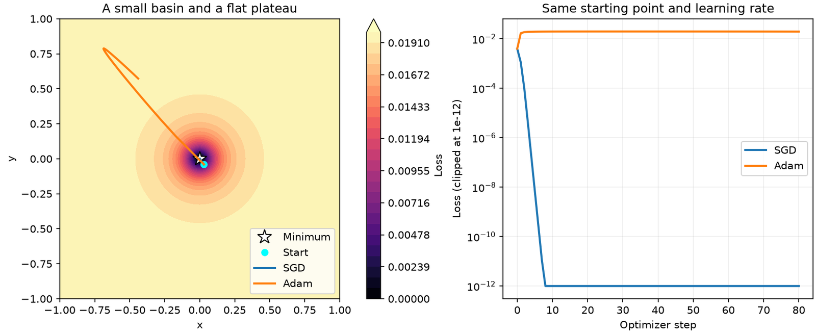
For readability, its logarithmic loss plot clips values below 1e−12. This is a visualization limit, not the actual numerical loss reached by SGD.
Why this is an instructive counterexample
The important result is not that SGD is universally better.
It is that adaptive normalization can remove useful information about absolute gradient magnitude.
Close to a minimum, a small gradient often signals that the optimizer should take a small step.
Plain gradient descent directly translates smaller gradients into smaller updates.
Adam’s step size depends on the ratio between its first- and second-moment estimates. In some regimes, this ratio can remain substantial even when the raw gradient becomes small.
That is useful when gradients are poorly scaled, but it can also cause undesirable movement when the appropriate physical step size is tiny.
The example is intentionally constructed to expose this limitation. A smaller Adam learning rate, a suitable learning-rate schedule, different initialization, or other tuning choices can change the result.
It does not establish that Adam is generally inferior. It demonstrates that optimizer behavior cannot be separated from the loss geometry and hyperparameter choices.
9. Interpreting convergence correctly
When comparing optimization algorithms, it is useful to distinguish three kinds of progress.
Parameter-space progress
This asks how close the current parameters are to a known optimum.
For our two-dimensional examples, we can directly measure distance to the optimal coordinates.
However, distance in parameter space is not always a reliable proxy for model quality. Some objectives contain broad regions of similarly low loss, and different parameter vectors can produce equivalent predictions.
Objective-space progress
This measures how much the loss decreases.
It is the primary metric in our figures because minimizing the objective is exactly what the optimizers are designed to do.
A useful comparison includes:
-
Final loss after a fixed update budget.
-
Best loss reached during optimization.
-
Number of updates required to cross a target loss.
-
Stability of the loss curve near the optimum.
Final loss and best loss are not always identical. An optimizer with a large learning rate may briefly reach a good region and then move away from it.
Computational progress
In practical systems, an iteration is not necessarily the same amount of work for every optimizer.
Momentum maintains an additional vector. RMSProp maintains squared-gradient statistics. Adam typically maintains both first- and second-moment vectors.
These states consume memory and require extra element-wise operations.
For a two-dimensional function, the overhead is negligible. For a large neural network, optimizer-state memory may become an important engineering constraint.
This is one reason a serious benchmark should consider memory footprint and elapsed training time as well as the final loss.
10. How to make this experiment more rigorous
Our race is designed for learning, but its structure also provides a foundation for controlled experiments.
Perform a learning-rate sweep
Instead of selecting one learning rate for each method, test several values spanning multiple orders of magnitude.
For every optimizer, record the best final loss under the same update budget.
This helps distinguish an algorithm’s limitations from a poorly chosen learning rate.
It is also worth logging diverged runs rather than silently ignoring them. A method that occasionally converges very quickly but diverges across many plausible settings has a different practical reliability profile from one that improves more slowly but consistently.
Change the initial coordinates
Move the starting point to other parts of the Rosenbrock surface.
Try positions above, below, and near the curved valley.
Momentum can behave differently when initialized with gradients that initially point across the valley rather than along it. Adam and RMSProp can also produce different early trajectories because their moving-average states are initialized to zero.
Measure threshold-crossing time
A useful metric is the number of gradient evaluations needed to reach a target loss.
For example, define success as reaching a loss below 0.01.
An optimizer that reaches that threshold after 200 steps may be preferable to one that has a slightly lower final loss after 1,000 steps, depending on the application.
This comparison is especially useful when optimizer trajectories intersect.
Add stochastic gradients
Our current functions return exact gradients.
In machine learning, stochastic optimization normally uses minibatches, producing gradient estimates that vary between iterations.
To experiment with noise, we could add independently generated random perturbations to the gradient using a seeded NumPy random generator.
That would allow us to investigate how momentum and adaptive second-moment estimates respond to gradient variance.
It would also require repeated trials across random seeds. A single noisy run would not provide enough evidence for a robust comparison.
11. Common mistakes when reproducing optimizer visualizations
Several small implementation details can change results substantially.
Forgetting Adam’s bias correction: With moving averages initialized at zero, omitting bias correction changes the early updates. It is not equivalent to the standard Adam algorithm used here.
Using the same learning rate without considering scaling: Adaptive and nonadaptive methods transform gradient information differently. Equal numerical learning rates do not necessarily imply comparable update magnitudes.
Mixing up squared-gradient history and gradient history: Momentum and Adam’s first moment track gradients. RMSProp and Adam’s second moment track squared gradients. Confusing these states changes the algorithms.
Updating optimizer state inside the animation callback: Animation frameworks can invoke the frame-rendering function more than once. This can silently make the number of optimizer steps depend on rendering behavior.
Using a linear color scale on a highly variable loss surface: Large loss values can hide the narrow valley. A logarithmic scale provides a clearer geometric picture, provided the plotted values are positive.
Interpreting a two-dimensional example as universal evidence: A synthetic surface isolates particular optimization behaviors. It cannot establish general superiority across neural networks, data distributions, and training objectives.
One additional detail matters when comparing this script with framework optimizers: RMSProp conventions and defaults can vary, and some implementations offer centered or momentum-enabled variants. Our implementation uses an uncentered, momentum-free RMSProp update, while our Adam implementation includes bias correction. These distinctions should be preserved in any reproduction.
12. What each optimizer teaches us
The main lessons extend beyond the particular numbers in our experiment.
| Optimizer | Main mechanism | Most important insight |
|---|---|---|
| SGD | Direct gradient updates | Gradient magnitude directly controls update magnitude |
| Momentum | Accumulated gradient history | Persistent directions can accelerate progress |
| RMSProp | Running squared-gradient average | Coordinate-wise normalization can help with unequal gradient scales |
| Adam | First and second moments | Adaptive updates are powerful but not universally safe |
Ordinary gradient descent remains an important baseline because it is simple to understand and diagnose. Its trajectory directly reflects the gradient field and learning rate.
Momentum shows how memory can improve optimization without requiring coordinate-wise adaptive scaling.
RMSProp demonstrates the practical value of adjusting effective learning rates according to recent gradient magnitude.
Adam illustrates how combining momentum and adaptive scaling can help navigate complicated objectives, while also introducing behavior that is less directly tied to the absolute gradient magnitude.
None of these mechanisms guarantees success in every setting.
The optimizer, learning rate, initialization, objective geometry, and available computational budget all interact.
13. Practical exercises to extend the visualization
Once you have the base script running, try these extensions.
-
Exercise 1 — Change momentum: Experiment with momentum coefficients of 0.5, 0.8, 0.9, and 0.99. Observe how the oscillations and final loss change.
-
Exercise 2 — Tune Adam: Sweep its learning rate over a range of values. Determine which settings escape the pathological plateau and which fail.
-
Exercise 3 — Increase the training budget: Run each optimizer for 2,000 steps. Investigate whether the performance ranking changes.
-
Exercise 4 — Compare coordinate scaling: Replace the Rosenbrock function with an anisotropic quadratic bowl, using different curvature in x and y.
-
Exercise 5 — Add a third visualization: Plot the distance from each optimizer’s current coordinates to the known global minimum.
-
Exercise 6 — Add Nesterov momentum: Implement a look-ahead gradient evaluation and compare its path with classical momentum.
-
Exercise 7 — Test learning-rate schedules: Reduce learning rates over time and observe whether oscillations near the minimum become smaller.
For a particularly interesting extension, animate the pathological plateau experiment itself.
Watch Adam’s first step carry it outside the low-loss basin, then compare its subsequent movement against SGD’s steady approach to the origin.
This visual makes the difference between gradient magnitude and normalized adaptive updates immediately apparent.
14. Final takeaways
The most important insight from our experiments is simple:
Optimization is not just about following gradients. It is about deciding how far to move, how much history to remember, and how to respond to changing geometry.
On our Rosenbrock surface, classical momentum produces the smallest final loss under the demonstrated configurations. Adam also makes substantial progress, while plain gradient descent and RMSProp follow different, less successful trajectories within the same 400-step budget.
On our pathological plateau, the outcome reverses dramatically. Plain SGD benefits from naturally shrinking steps as it approaches the minimum, while Adam’s initially normalized update overshoots the narrow basin and leaves it struggling on a nearly flat surface.
These results do not identify a universally best optimizer. They reveal why no such simple choice exists.
A good practical approach is to understand the update rule, examine the objective and gradient scales, tune the learning rate, and evaluate convergence instead of choosing solely by reputation.
Your next step: Run the script, open the animated GIF, and change one hyperparameter at a time. Start with Adam’s learning rate on the pathological surface, then experiment with momentum on the Rosenbrock valley.
Watch how a small change in step size reshapes an entire optimization trajectory.
That is where gradient-based optimization stops being a collection of formulas and becomes something you can reason about visually.