
LEARN · EXPLORATORY DATA ANALYSIS & STATISTICS
A service can have the same average latency, the same standard deviation, and the same request volume as yesterday—and still deliver a dramatically different user experience.
Imagine two versions of an API. Version A responds at reasonably consistent speeds. Version B has developed two distinct operating modes: requests either finish unusually quickly or become noticeably slow. Their averages might match, but their latency distributions tell different stories.
This is exactly the kind of problem that distribution tests help uncover.
The Kolmogorov–Smirnov (K-S) test compares cumulative distributions rather than just their summary statistics. It can identify changes in location, spread, skewness, or shape without requiring us to decide in advance which of those characteristics might have changed.
In this tutorial, we’ll build a practical toolkit around three complementary ideas:
-
One-sample K-S: Does a dataset agree with a specified probability distribution?
-
Two-sample K-S: Could two independent datasets have come from the same continuous distribution?
-
Anderson–Darling: How can we test goodness of fit while giving greater attention to differences in the distribution tails?
We’ll implement the tests using modern SciPy, examine their mathematical foundations, solve the tricky problem of fitting distribution parameters, and finish with a reproducible experiment in which two datasets have identical sample means and standard deviations but a statistically detectable difference in shape.
1. Why comparing averages is not enough
Consider a monitoring system collecting API response times.
The first dashboard shows:
| Metric | Baseline | New deployment |
|---|---|---|
| Mean latency | 100 ms | 100 ms |
| Standard deviation | 30 ms | 30 ms |
| Request volume | 10,000 | 10,000 |
At first glance, everything appears stable.
But these metrics leave out crucial information.
For example, the new deployment might produce more very fast responses and more slow responses, while generating fewer responses near the average.
Two distributions can share their first two moments—mean and variance—yet differ substantially in their probability density, quantiles, and cumulative probabilities.
This matters in many domains:
-
Software operations: A change in response-time distribution may indicate performance regressions.
-
E-commerce: Average order values may remain unchanged while purchasing behavior shifts toward very small and very large orders.
-
Manufacturing: Sensor readings may develop multiple operating modes even when the overall variance remains stable.
-
Machine learning: Incoming feature distributions may change without noticeably affecting their averages.
-
Energy systems: Consumption patterns may shift between peak and off-peak periods despite unchanged average usage.
A mean comparison cannot detect every type of change. Neither can a variance comparison.
To identify more general distributional differences, we need to examine how probability accumulates across the entire range of observed values.
That’s where empirical cumulative distribution functions come in.
2. The empirical cumulative distribution function
The cumulative distribution function, or CDF, of a random variable X is:
F(x) = P(X ≤ x)
It answers a simple question:
What proportion of the probability distribution lies at or below a particular value?
For example, if the latency CDF at 120 milliseconds is 0.80, then 80% of requests take at most 120 milliseconds.
When we do not know the true distribution, we estimate the CDF directly from the sample.
This is called the empirical cumulative distribution function, or ECDF.
For observations x₁, x₂, …, xₙ:
F̂ₙ(t) = (number of observations ≤ t) / n
The ECDF is a step function. Every observation increases the cumulative proportion by 1/n, counting repeated observations separately.
Let’s implement one without a statistics library.
import numpy as np

def ecdf(sample, thresholds):
    sample = np.sort(np.asarray(sample))
    thresholds = np.asarray(thresholds)

    counts = np.searchsorted(
        sample,
        thresholds,
        side="right"
    )

    return counts / sample.size


latencies = np.array([
    80, 90, 90, 100, 110,
    120, 120, 120, 140, 160
])

thresholds = np.array([90, 120, 150])

probabilities = ecdf(latencies, thresholds)

for threshold, probability in zip(
    thresholds,
    probabilities
):
    print(
        f"P(latency <= {threshold}) "
        f"= {probability:.2f}"
    )
Output:
P(latency <= 90) = 0.30
P(latency <= 120) = 0.80
P(latency <= 150) = 0.90
Notice that three observations have the value 120. The ECDF therefore makes a larger jump at that point.
An ECDF preserves much more distributional information than a mean or standard deviation.
We can now compare two ECDFs—or one ECDF against a theoretical CDF—to measure how far apart the distributions are.
3. The Kolmogorov–Smirnov statistic: the maximum vertical gap
The central idea behind the K-S test is remarkably simple.
Find the largest absolute vertical distance between two cumulative distribution functions.
For a one-sample test, the statistic is:
Dₙ = supₓ |F̂ₙ(x) − F₀(x)|
Here:
-
F̂ₙ(x) is the empirical CDF calculated from the data.
-
F₀(x) is the proposed theoretical CDF.
-
supₓ means the largest value over all x.
-
Dₙ is the maximum absolute difference between the curves.
For a two-sample test, the statistic becomes:
Dₙ,ₘ = supₓ |F̂ₙ(x) − Ĝₘ(x)|
Now both CDFs come from observed samples.
The K-S statistic always lies between 0 and 1.
A value of 0 means the compared CDFs coincide everywhere. A value of 0.20 means that at some threshold, their cumulative proportions differ by 20 percentage points.
That interpretation makes D useful as an effect-size-like measure of distributional separation.
Importantly, D is not itself a p-value.
The significance of a particular D depends on the sample sizes, the hypothesis, and the assumptions used to calculate its null distribution.
Calculating D manually
Let’s compare four observations against the uniform distribution between 0 and 1.
For sorted observations, we must examine the discrepancy both immediately before and immediately after every ECDF jump.
The two one-sided components are:
D⁺ = maxᵢ [i/n − F₀(xᵢ)]
D⁻ = maxᵢ [F₀(xᵢ) − (i−1)/n]
The two-sided statistic is:
D = max(D⁺, D⁻)
Here’s a complete implementation:
import numpy as np
from scipy import stats

sample = np.array([0.1, 0.4, 0.5, 0.9])

x = np.sort(sample)
n = len(x)

theoretical_cdf = stats.uniform.cdf(x)

d_plus = np.max(
    np.arange(1, n + 1) / n
    - theoretical_cdf
)

d_minus = np.max(
    theoretical_cdf
    - np.arange(n) / n
)

manual_d = max(d_plus, d_minus)

scipy_result = stats.ks_1samp(
    sample,
    stats.uniform.cdf,
    method="exact"
)

print(f"Manual D: {manual_d:.4f}")
print(f"SciPy D:  {scipy_result.statistic:.4f}")
print(f"p-value:  {scipy_result.pvalue:.5f}")
Output:
Manual D: 0.2500
SciPy D:  0.2500
p-value:  0.90625
The manual implementation and SciPy agree.
An easy mistake is to compare the theoretical CDF only against i/n at each observation. That misses discrepancies immediately before ECDF jumps and can underestimate the statistic.
The NIST goodness-of-fit reference explicitly documents this distinction.
4. Setting up the Python environment
We’ll use NumPy for arrays and simulation, SciPy for statistical testing, and Matplotlib for visual inspection.
The examples use synthetic data, so no downloads, credentials, API connections, or external datasets are required.
Create a virtual environment:
python -m venv .venv
source .venv/bin/activate

python -m pip install --upgrade pip
python -m pip install "numpy>=2.0" "scipy>=1.17" "matplotlib>=3.10"
You can verify the installed versions:
python -c "import numpy, scipy; print(numpy.__version__, scipy.__version__)"
The examples use current SciPy interfaces, including the newer Anderson–Darling p-value options and the rng keyword for reproducible simulation.
5. One-sample K-S: testing against a theoretical distribution
The one-sample K-S test evaluates the hypothesis that observations come from a particular, fully specified continuous distribution.
Formally:
H₀: The observations follow the specified distribution F₀.
H₁: The observations do not follow F₀.
Suppose an API performance model predicts that response times follow a lognormal distribution.
A lognormal distribution is a reasonable illustrative model for nonnegative, right-skewed latency data.
For this first experiment, assume the model parameters have been specified in advance, rather than estimated using the observations we’re testing.
import numpy as np
from scipy import stats

rng = np.random.default_rng(101)

# Synthetic response times, in milliseconds
latencies = rng.lognormal(
    mean=4.5,
    sigma=0.35,
    size=350
)

# Hypothesized distribution, specified in advance
expected = stats.lognorm(
    s=0.35,
    scale=np.exp(4.5)
)

result = stats.ks_1samp(
    latencies,
    expected.cdf,
    alternative="two-sided",
    method="auto"
)

print(f"K-S statistic: {result.statistic:.4f}")
print(f"p-value:       {result.pvalue:.4f}")
print(
    f"Largest gap at: "
    f"{result.statistic_location:.2f} ms"
)
print(f"Gap direction: {result.statistic_sign:+d}")
With the specified seed, the statistic is approximately 0.0562 and the p-value is approximately 0.211.
At the conventional 5% significance level, we would not reject the null hypothesis.
That does not prove the data follow the lognormal distribution. It means this particular sample does not provide sufficiently strong evidence against the stated model.
Understanding the result object
SciPy’s ks_1samp returns more than a statistic and p-value.
Its result includes:
| Attribute | Interpretation |
|---|---|
statistic |
Maximum absolute CDF gap |
pvalue |
Statistical significance under the test assumptions |
statistic_location |
Observation where the maximum discrepancy occurs |
statistic_sign |
Direction of the empirical-versus-theoretical CDF difference |
The location is especially useful operationally.
A significant discrepancy around 100 milliseconds may have a different implication from a discrepancy around 2,000 milliseconds.
However, the maximum-gap location is just one part of the distributional picture. Other important differences may occur elsewhere.
The one-sample K-S test is available through SciPy’s documented ks_1sampinterface.
6. The parameter-fitting trap: why a naive K-S p-value can be wrong
This is one of the most important subtleties in goodness-of-fit testing.
Suppose we want to determine whether a dataset follows a normal distribution.
A natural workflow is:
-
Estimate the mean and standard deviation from the observations.
-
Construct a normal distribution using those estimates.
-
Compare the observations against the fitted normal CDF.
Calculating the K-S statistic this way is entirely legitimate.
But interpreting its ordinary p-value as though the normal distribution had been fully specified before observing the data is not.
Why?
Because fitting the parameters to the same sample makes the theoretical CDF unusually close to that sample.
The null distribution of the resulting K-S statistic is therefore different from the ordinary one-sample K-S null distribution.
This is related to the classical Lilliefors problem.
The naive approach
Let’s generate sensor readings from a uniform distribution and see whether they appear normally distributed.
import numpy as np
from scipy import stats

rng = np.random.default_rng(35)

readings = rng.uniform(
    low=-1,
    high=1,
    size=250
)

# Fit a normal distribution to the test data
loc, scale = stats.norm.fit(readings)

fitted_normal = stats.norm(
    loc=loc,
    scale=scale
)

naive = stats.ks_1samp(
    readings,
    fitted_normal.cdf
)

print(f"Fitted mean: {loc:.4f}")
print(f"Fitted std:  {scale:.4f}")
print(f"K-S D:       {naive.statistic:.4f}")
print(f"Naive p:     {naive.pvalue:.6f}")
The ordinary p-value is approximately 0.0263.
But this p-value uses the wrong null calibration for a test of the whole normal family with unknown parameters.
It’s not enough to choose method="exact" or method="asymp". Neither option automatically accounts for the parameters estimated from the same sample.
The correct approach: Monte Carlo calibration with refitting
SciPy provides stats.goodness_of_fit, which handles unknown distribution parameters through a Monte Carlo procedure.
Conceptually, it:
-
Fits the proposed distribution family to the observed data.
-
Generates samples from the fitted null distribution.
-
Refits the unknown parameters separately for every simulated sample.
-
Computes the goodness-of-fit statistic for every simulation.
-
Compares the observed statistic with the resulting Monte Carlo null distribution.
The crucial step is number three.
Every simulated dataset gets the same fitting treatment as the original dataset.
import numpy as np
from scipy import stats

rng = np.random.default_rng(35)

readings = rng.uniform(
    low=-1,
    high=1,
    size=250
)

result = stats.goodness_of_fit(
    stats.norm,
    readings,
    statistic="ks",
    n_mc_samples=1999,
    rng=np.random.default_rng(85)
)

print(f"Corrected K-S D: {result.statistic:.4f}")
print(f"Monte Carlo p:   {result.pvalue:.6f}")
print(f"Simulations:     {len(result.null_distribution)}")
The calibrated p-value is 0.0005.
That is the smallest p-value resolvable by this particular 1,999-resample configuration.
The result provides strong evidence that these uniformly generated observations do not come from a normal distribution.
Notice that the observed K-S statistic may differ slightly from the previous example: goodness_of_fit applies its own documented fitting convention for a normal distribution with unknown mean and scale.
SciPy’s goodness-of-fit documentation explains the refitting procedure and why treating estimated parameters as known can produce misleadingly conservative p-values.
When should you use each approach?
Use ks_1samp with its standard p-value when the comparison CDF is fully specified independently of the tested observations.
Use goodness_of_fit when you’re testing membership in a distribution family and fitting unknown parameters from the tested sample.
If parameters were estimated from an independent calibration sample, that removes the same-sample fitting problem but does not automatically eliminate parameter uncertainty. A fully calibrated procedure may still need to account for the independent estimation stage.
7. Two-sample K-S: detecting distribution changes
The two-sample K-S test is particularly useful for distribution monitoring.
Rather than comparing observations against a theoretical distribution, it compares two empirical CDFs.
The hypotheses are:
H₀: Both independent samples come from the same underlying continuous distribution.
H₁: The underlying distributions differ.
We do not need to assume that either sample follows a normal, lognormal, or another specific parametric family.
This is why the test is often called nonparametric.
A reproducible distribution-shift experiment
We’ll compare two kinds of simulated system behavior.
The baseline comes from a standard normal distribution.
The second dataset comes from a mixture of two normal operating modes. It is deliberately constructed to have the same theoretical mean and variance as the baseline.
import numpy as np
from scipy import stats

rng = np.random.default_rng(2026)

n = 1200

# Baseline: one operating mode
baseline = rng.normal(
    loc=0,
    scale=1,
    size=n
)

# Changed system: two operating modes
offset = 0.92
noise_scale = np.sqrt(1 - offset**2)

changed = (
    rng.choice([-1.0, 1.0], size=n) * offset
    + rng.normal(scale=noise_scale, size=n)
)

result = stats.ks_2samp(
    baseline,
    changed,
    alternative="two-sided",
    method="auto"
)

print(f"Baseline mean: {baseline.mean():.4f}")
print(f"Changed mean:  {changed.mean():.4f}")

print(
    f"Baseline std: "
    f"{baseline.std(ddof=1):.4f}"
)
print(
    f"Changed std:  "
    f"{changed.std(ddof=1):.4f}"
)

print(f"K-S D:    {result.statistic:.4f}")
print(f"p-value:  {result.pvalue:.3e}")
print(
    f"Max gap:  "
    f"{result.statistic_location:.4f}"
)
The generated samples have approximately the same scale and similar means.
More importantly, both generating distributions have exactly the same theoretical mean of 0 and variance of 1.
For the mixture, the variance is:
Variance = offset² + noise_scale² = 0.92² + (1 − 0.92²) = 1
Despite this, the two-sample K-S statistic is approximately 0.1467, with a p-value around 1.13 × 10⁻¹¹.
The distribution change is statistically unmistakable.
The result’s statistic_location tells us where the empirical cumulative proportions differ most. The statistic_sign tells us which sample has the larger ECDF at that location.
The key takeaway is that matching population means and variances does not imply matching probability distributions.
Verifying the two-sample statistic manually
We can calculate both ECDFs at every observed value in the combined sample.
import numpy as np
from scipy import stats

rng = np.random.default_rng(123)

baseline = rng.normal(size=200)
changed = rng.normal(
    loc=0.5,
    size=200
)

grid = np.sort(
    np.concatenate([baseline, changed])
)

sorted_baseline = np.sort(baseline)
sorted_changed = np.sort(changed)

cdf_baseline = (
    np.searchsorted(
        sorted_baseline,
        grid,
        side="right"
    ) / len(baseline)
)

cdf_changed = (
    np.searchsorted(
        sorted_changed,
        grid,
        side="right"
    ) / len(changed)
)

manual_d = np.max(
    np.abs(cdf_baseline - cdf_changed)
)

scipy_d = stats.ks_2samp(
    baseline,
    changed
).statistic

print(f"Manual D: {manual_d:.6f}")
print(f"SciPy D:  {scipy_d:.6f}")

assert np.isclose(manual_d, scipy_d)
The maximum difference occurs at one of the observed sample values.
This is why we can calculate the statistic using the finite set of sample observations, even though its mathematical definition considers every real-valued threshold.
8. Visualizing where distributions separate
A numerical test tells us whether the evidence suggests a difference. An ECDF plot helps us understand what that difference looks like.
Using the same mixture scenario, let’s draw both curves and mark the location of their largest separation.
import numpy as np
import matplotlib.pyplot as plt
from scipy import stats

rng = np.random.default_rng(2026)

n = 1200
offset = 0.92
noise_scale = np.sqrt(1 - offset**2)

baseline = rng.normal(size=n)

changed = (
    rng.choice([-1.0, 1.0], size=n) * offset
    + rng.normal(scale=noise_scale, size=n)
)

def ecdf_points(values):
    ordered = np.sort(values)
    probabilities = (
        np.arange(1, len(ordered) + 1)
        / len(ordered)
    )

    return ordered, probabilities

x1, y1 = ecdf_points(baseline)
x2, y2 = ecdf_points(changed)

result = stats.ks_2samp(
    baseline,
    changed
)

fig, ax = plt.subplots(figsize=(9, 5))

ax.step(
    x1, y1,
    where="post",
    label="Baseline"
)

ax.step(
    x2, y2,
    where="post",
    label="Changed system"
)

ax.axvline(
    result.statistic_location,
    linestyle="--",
    color="black",
    alpha=0.6,
    label="Largest CDF gap"
)

ax.set_title(
    f"ECDF comparison: D = {result.statistic:.3f}"
)

ax.set_xlabel("Standardized operating metric")
ax.set_ylabel("Cumulative probability")
ax.set_ylim(0, 1)

ax.legend()
ax.grid(alpha=0.2)

fig.tight_layout()
fig.savefig("ecdf_comparison.png", dpi=160)

plt.show()
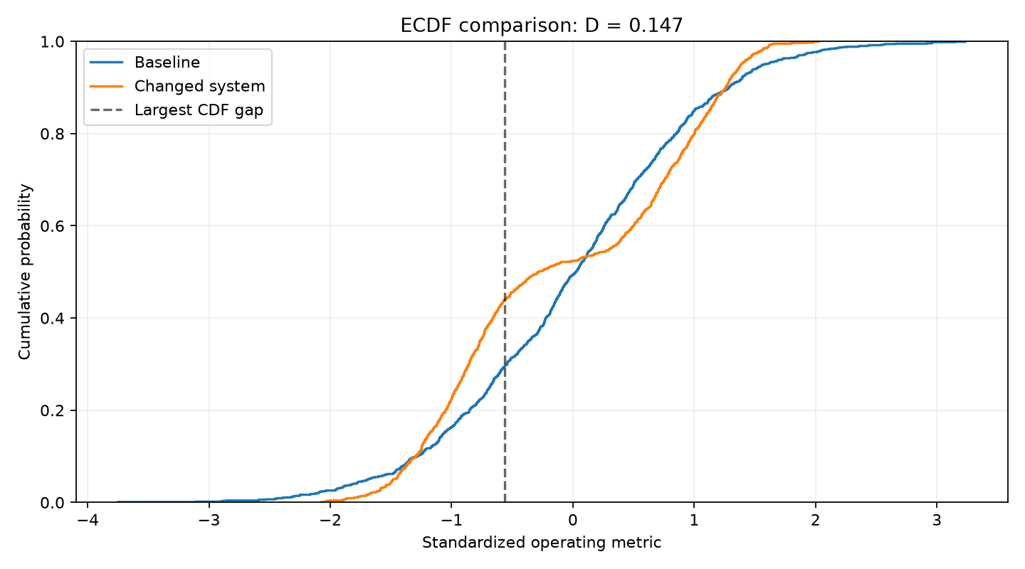
The changed distribution has a different ECDF shape, with areas where probability accumulates more quickly or more slowly.
For a continuous distribution, the one-dimensional K-S statistic is insensitive to the units of measurement under a shared strictly increasing transformation applied to both samples.
For example, changing latency units from milliseconds to seconds does not change the statistic.
This is useful when comparing measurements across compatible systems.
However, a K-S test cannot explain why a distribution changed. It provides evidence of a difference, not a causal diagnosis.
9. Anderson–Darling: giving the tails more attention
The Kolmogorov–Smirnov statistic looks only at the largest vertical CDF gap.
That makes it straightforward to interpret, but it also means the test is not equally sensitive to every kind of discrepancy.
In particular, classical K-S tests often have less power for differences concentrated in the tails than for differences near the center of a distribution.
The Anderson–Darling (A-D) test takes a different approach.
Instead of measuring only the maximum difference, it aggregates discrepancies across the distribution while assigning greater weight to observations in regions where the reference CDF approaches 0 or 1.
This makes Anderson–Darling especially useful when unusual extreme values matter.
Consider applications such as:
-
Very slow API responses.
-
Unexpectedly large e-commerce orders.
-
Extreme sensor measurements.
-
Unusually high electricity consumption.
One-sample Anderson–Darling
We’ll revisit the uniform sensor readings and test the hypothesis that they come from a normal distribution.
The current SciPy interface allows an explicit method for obtaining an Anderson–Darling p-value.
import numpy as np
from scipy import stats

rng = np.random.default_rng(35)

readings = rng.uniform(
    low=-1,
    high=1,
    size=250
)

result = stats.anderson(
    readings,
    dist="norm",
    method="interpolate"
)

print(f"A-D statistic: {result.statistic:.4f}")
print(f"p-value:       {result.pvalue:.6f}")
The test returns a statistic around 4.2062 and an interpolated p-value of 0.01.
That p-value should not be treated as an exact measurement here. The table-based calculation has a limited reported range.
For a more detailed Monte Carlo estimate:
import numpy as np
from scipy import stats

rng = np.random.default_rng(35)

readings = rng.uniform(
    low=-1,
    high=1,
    size=250
)

result = stats.goodness_of_fit(
    stats.norm,
    readings,
    statistic="ad",
    n_mc_samples=1999,
    rng=np.random.default_rng(86)
)

print(f"A-D statistic: {result.statistic:.4f}")
print(f"Monte Carlo p: {result.pvalue:.6f}")
This produces a Monte Carlo p-value of 0.0005.
For normality testing, SciPy’s Anderson–Darling implementation accounts for the normal parameters being estimated from the observations, rather than simply assuming a standard normal distribution with fixed parameters.
The newer method argument also avoids relying on legacy result attributes that SciPy is deprecating.
Two-sample Anderson–Darling
There is also an Anderson–Darling extension for comparing two or more samples.
SciPy exposes this through stats.anderson_ksamp.
We can compare our two operating modes using a permutation-calibrated p-value.
import numpy as np
from scipy import stats

rng = np.random.default_rng(2026)

n = 1200
offset = 0.92

baseline = rng.normal(size=n)

changed = (
    rng.choice([-1.0, 1.0], size=n) * offset
    + rng.normal(
        scale=np.sqrt(1 - offset**2),
        size=n
    )
)

method = stats.PermutationMethod(
    n_resamples=1999,
    rng=np.random.default_rng(333)
)

result = stats.anderson_ksamp(
    [baseline, changed],
    variant="midrank",
    method=method
)

print(f"A-D statistic: {result.statistic:.4f}")
print(f"Permutation p: {result.pvalue:.6f}")
The result provides strong evidence that the samples have different distributions.
Unlike the two-sample K-S statistic, the normalized k-sample Anderson–Darling statistic is not a maximum cumulative-probability gap. Its numerical size should not be interpreted as a percentage or compared directly against a K-S D value.
The variant argument is the current explicit way to choose the Anderson–Darling k-sample formulation. The older midrank parameter is deprecated in recent SciPy releases.
10. Cherry on the cake: identical means and variances, but a detectable shift
There is a famous published demonstration of how unreliable simple summary statistics can be.
In 2017, Justin Matejka and George Fitzmaurice published Same Stats, Different Graphs, introducing the Datasaurus Dozen.
They constructed dramatically different datasets—including one shaped like a dinosaur—while preserving nearly identical means, standard deviations, and correlations to two decimal places.
The datasets were designed to show that numerical summaries can conceal substantial structural differences. They were not a documented production incident detected by K-S, and not every difference in a two-dimensional dataset can be detected by examining one-dimensional marginals.
We can demonstrate the corresponding one-dimensional lesson directly, using K-S.
This experiment goes further than matching theoretical population moments: we’ll make the observed sample means and standard deviations equal by construction.
There is one subtle statistical complication.
Standardizing each sample separately affects the null distribution of the K-S statistic. We should therefore not blindly use the ordinary K-S p-value after that preprocessing.
Instead, we’ll calculate a shape-only maximum ECDF gap and calibrate it using a permutation test that repeats the standardization for every permutation.
Step 1: Generate two differently shaped samples
The baseline is normal. The changed system is a two-mode mixture.
Step 2: Match their sample mean and standard deviation
We subtract each sample mean and divide by its sample standard deviation.
Both transformed samples then have mean 0 and sample standard deviation 1, up to floating-point precision.
Step 3: Test the residual shape difference
We’ll recompute the normalized gap for randomly reassigned group labels.
import numpy as np
from scipy import stats

rng = np.random.default_rng(2026)

n = 1200
offset = 0.92
noise_scale = np.sqrt(1 - offset**2)

baseline = rng.normal(size=n)

changed = (
    rng.choice([-1.0, 1.0], size=n) * offset
    + rng.normal(scale=noise_scale, size=n)
)

def standardize(values):
    return (
        (values - values.mean())
        / values.std(ddof=1)
    )

def shape_gap(sample_a, sample_b):
    a = standardize(sample_a)
    b = standardize(sample_b)

    return stats.ks_2samp(
        a,
        b,
        method="asymp"
    ).statistic

# Examine the standardized observations
a = standardize(baseline)
b = standardize(changed)

print("Standardized summaries:")

print(
    f"A: mean={a.mean():.6f}, "
    f"std={a.std(ddof=1):.6f}"
)

print(
    f"B: mean={b.mean():.6f}, "
    f"std={b.std(ddof=1):.6f}"
)

# Recalculate both standardization and
# the K-S gap for every permutation.
result = stats.permutation_test(
    (baseline, changed),
    shape_gap,
    permutation_type="independent",
    alternative="greater",
    vectorized=False,
    n_resamples=1999,
    rng=np.random.default_rng(444)
)

print(f"Shape-only D: {result.statistic:.6f}")
print(f"Permutation p: {result.pvalue:.6f}")
Representative output from the specified seeds:
Standardized summaries:
A: mean=-0.000000, std=1.000000
B: mean=-0.000000, std=1.000000

Shape-only D: 0.129167
Permutation p: 0.000500
The negative zeros are floating-point formatting artifacts, not meaningful differences.
The results are striking.
Both standardized samples have the same mean and standard deviation.
Yet their empirical CDFs differ by almost 13 percentage points at the point of greatest separation.
The permutation-calibrated p-value provides strong evidence of a distributional difference.
Why is the permutation calibration important?
Under the null hypothesis of independent, identically distributed observations, the original group labels are exchangeable. Each permutation reproduces the entire analysis procedure, including recalculating each sample’s mean and standard deviation.
This creates an appropriate reference distribution for our specifically defined shape-only statistic.
Had we standardized each group once and simply reported the ordinary ks_2samp p-value, we would have ignored the effect of the fitted normalization.
The lesson: matching means and variances—even exactly at the sample level—does not guarantee matching distributions.
This matters whenever dashboards, model monitors, or business reports reduce complex populations to a handful of summary statistics.
11. Choosing the right goodness-of-fit test
No single test is uniformly best for every possible alternative distribution.
The choice should reflect what you are comparing, the assumptions you can justify, and the kinds of differences that matter.
| Test | Main purpose | Strength | Important limitation |
|---|---|---|---|
| One-sample K-S | Sample versus specified CDF | Interpretable maximum gap | Parameter fitting requires separate calibration |
| Two-sample K-S | Two independent samples | General shape-shift detection | Classical p-values assume continuous distributions |
| One-sample A-D | Sample versus distribution family | Greater tail sensitivity | Available reference families and calibration methods vary |
| K-sample A-D | Two or more samples | Tail-sensitive multi-sample comparison | Statistic is less directly interpretable |
| Cramér–von Mises | Integrated CDF discrepancy | Uses differences across the CDF | Less immediately interpretable than maximum gap |
| Wasserstein distance | Distributional distance | Expressed in measurement units | Distance alone does not provide a hypothesis-test p-value |
Cramér–von Mises as another alternative
If the goal is to detect smaller differences spread across the CDF, Cramér–von Mises may be useful.
SciPy supports it through the same fitted-family testing interface:
import numpy as np
from scipy import stats

rng = np.random.default_rng(42)

readings = rng.uniform(
    low=-1,
    high=1,
    size=250
)

result = stats.goodness_of_fit(
    stats.norm,
    readings,
    statistic="cvm",
    n_mc_samples=1999,
    rng=np.random.default_rng(99)
)

print(f"CvM statistic: {result.statistic:.4f}")
print(f"p-value:       {result.pvalue:.6f}")
This is a useful reminder that the K-S statistic is only one possible way to summarize discrepancies between cumulative distributions.
12. Common mistakes that invalidate distribution testing
The mathematical simplicity of K-S can make it deceptively easy to misuse.
Mistake 1: Treating a large p-value as proof of equality
A non-significant result does not establish that two distributions are identical.
It may indicate that the sample was too small to reveal a real difference.
Failure to reject H₀ is not the same as demonstrating equivalence.
If the business goal is to establish that two distributions are sufficiently similar, define an acceptable difference threshold and consider an equivalence-testing or confidence-bound approach designed for that purpose.
Mistake 2: Ignoring the independence assumption
Standard K-S significance calculations assume independent observations.
Real telemetry is often temporally correlated.
For example, 50,000 latency measurements collected during a persistent slowdown are not necessarily equivalent to 50,000 independent observations.
If measurements come from correlated sessions, machines, or time blocks, consider sampling independent units or using resampling methods that preserve the relevant dependence.
Ordinary permutation tests are not automatically valid for arbitrary time series.
Mistake 3: Applying continuous K-S calibration to discrete data
Classical K-S null distributions are derived for continuous underlying distributions.
Data with genuine discreteness or substantial ties can violate those assumptions.
Examples include integer-valued star ratings, rounded counts, and heavily quantized measurements.
For discrete observations, consider a test designed for the discrete setting or a correctly constructed permutation procedure.
SciPy’s k-sample Anderson–Darling midrank variant is one possible alternative for comparisons involving ties, subject to the study design and independence assumptions.
Mistake 4: Ignoring sample size
With millions of observations, even a tiny and operationally irrelevant distributional difference can produce a very small p-value.
Always examine both statistical significance and practical magnitude.
For example:
-
D = 0.005 corresponds to a maximum cumulative-probability difference of half a percentage point.
-
D = 0.10 corresponds to a maximum cumulative-probability difference of ten percentage points.
Whether either difference matters depends on the application and where it occurs.
These D values are descriptive; they do not themselves establish significance.
Mistake 5: Repeating tests without accounting for multiplicity
Suppose a monitoring system performs 500 independent hypothesis tests under true null hypotheses, each at a 5% significance level.
The expected number of false rejections is 25.
Correlations between tests affect the joint behavior, but repeated testing still creates a multiple-comparisons problem.
For many simultaneous features, consider procedures such as Holm correction or Benjamini–Hochberg false-discovery-rate control.
Repeated daily monitoring also requires thought about sequential testing and alert policies.
Mistake 6: Assuming a marginal test detects every multivariate shift
A one-dimensional K-S test examines one variable at a time.
Two multivariate datasets can have identical distributions for every individual feature while differing in how those features interact.
For example, the relationship between temperature and electricity consumption could change while their individual marginal distributions remain the same.
Marginal K-S tests cannot establish equality of a joint distribution.
For multivariate monitoring, consider dependence measures, carefully designed projection tests, energy distances, or kernel-based methods.
13. A practical workflow for production distribution monitoring
A sensible monitoring system should combine hypothesis testing with effect-size reporting, visual inspection, and engineering judgment.
A useful workflow is:
-
Define the population. Compare the same metric, units, traffic segment, and measurement protocol.
-
Choose a reference. Use a representative baseline window or a sufficiently justified theoretical distribution.
-
Inspect data quality. Check missing values, rounding, duplicates, truncation, and unit changes.
-
Check dependence. Determine whether observations can reasonably be treated as independent.
-
Visualize ECDFs. Look at where and how the curves separate.
-
Select a calibrated test. Use K-S for general continuous distribution comparisons, and consider A-D where tails are especially important.
-
Report more than a p-value. Include the statistic, sample sizes, location of the largest discrepancy, and relevant quantiles.
-
Account for repeated monitoring. Avoid treating each alert opportunity as an isolated experiment.
-
Investigate operational causes. Stratify by region, version, instance type, customer segment, or workload where appropriate.
For example, an API monitoring report could contain:
| Signal | Example finding | Operational interpretation |
|---|---|---|
| Mean | Stable | Average performance has not obviously changed |
| Standard deviation | Stable | Overall spread appears similar |
| K-S statistic | 0.13 | Maximum ECDF separation is 13 percentage points |
| K-S p-value | Below 0.001 | Strong evidence against equal distributions under assumptions |
| P95 latency | Increased | Slower requests may deserve investigation |
| A-D comparison | Significant | Additional evidence of a distributional change |
This is much more informative than a binary pass/fail result.
A low p-value should prompt investigation, not automatically trigger a rollback. The operational impact, likely cause, reproducibility, and potential measurement artifacts still matter.
14. Final takeaways
The Kolmogorov–Smirnov test offers a remarkably compact answer to a broad statistical question: how far apart are two cumulative distributions at their most different point?
But using the test correctly requires more than calling a SciPy function.
Remember the essential distinctions:
-
The K-S statistic measures a maximum CDF gap. It is not a difference of means, a variance ratio, or a p-value.
-
One-sample K-S compares observations against a specified theoretical distribution. Parameters estimated from the tested data require appropriate calibration.
-
Two-sample K-S compares independent empirical distributions. It is particularly useful for detecting general changes in continuous measurements.
-
Anderson–Darling is a valuable complement. It can be more sensitive to tail discrepancies that matter in operational risk and reliability.
-
Permutation and Monte Carlo methods make distribution testing more flexible. But the simulation must reproduce the full analysis procedure and respect the data’s dependence structure.
-
Matching summary statistics does not imply matching distributions. Our final experiment demonstrated that even exact matching of sample means and standard deviations can leave a highly detectable difference in distributional shape.
For further technical details, consult the current SciPy statistical testing documentation, the NIST goodness-of-fit handbook, and the Datasaurus research paper.
Put it into practice
Pick one important numerical metric from a system you work with—API latency, transaction size, sensor output, or model feature values—and compare two independent samples from different periods.
Plot their ECDFs, run stats.ks_2samp, inspect the maximum-gap location, and repeat the analysis with stats.anderson_ksamp.
Then compare those findings against what the mean and standard deviation alone would have told you.
The goal is not simply to produce another p-value. It’s to uncover meaningful behavior that ordinary dashboards might otherwise miss.
Start measuring the shape of your data, not just its average.