
LEARN · MULTI-MODEL INFERENCE & SERVING
A model that achieves 92% accuracy in 2 milliseconds may be more valuable in production than an ensemble that achieves 93% accuracy in 40 milliseconds. But what if the ensemble reaches 95%? And what if combining two models provides almost the same improvement as combining ten?
These are the questions that make inference-time ensembling an engineering decision rather than simply a machine learning technique.
Ensembling combines predictions from multiple models to produce a final prediction. It is one of the most reliable ways to improve predictive performance, especially when the models make different kinds of mistakes.
The trade-off is straightforward: every additional model consumes computation, memory, and potentially network resources. A technique that improves an offline benchmark can become an expensive liability in a latency-sensitive application.
In this tutorial, we’ll build and benchmark several classification approaches using Python and scikit-learn:
-
Individual models: Establish performance and latency baselines.
-
Hard voting: Combine class predictions using majority rule.
-
Soft voting: Average predicted probabilities, optionally assigning different weights to each model.
-
Stacking: Train a second-level model to learn how the base models’ predictions should be combined.
-
Cost-aware model selection: Compare accuracy improvements against additional inference latency.
We’ll use a reproducible synthetic dataset representing a generic binary classification problem, such as predicting whether a retail order requires manual review. No external dataset download is necessary.
By the end, you’ll have a runnable benchmarking experiment, a practical framework for evaluating ensembles, and a better understanding of when extra predictive accuracy justifies the added serving cost.
1. Why inference-time ensembling works
Imagine three models predicting whether an e-commerce transaction requires additional review.
| Model | Predicted probability of review |
|---|---|
| Logistic regression | 0.35 |
| Random forest | 0.72 |
| Histogram-based gradient boosting | 0.81 |
The models disagree. Logistic regression predicts that review is unnecessary, while the two tree-based models lean toward review.
A hard-voting ensemble predicts review because two of the three models vote for that class.
A soft-voting ensemble averages the probabilities:
Average probability = (0.35 + 0.72 + 0.81) / 3 = 0.627
Because 0.627 exceeds a decision threshold of 0.5, the soft-voting ensemble also predicts review.
However, the two strategies are not equivalent.
Hard voting treats each model’s final class prediction as one vote. Soft voting considers the strength of each model’s predicted probability.
A stacking ensemble goes further. Instead of manually deciding how to combine predictions, it learns a combination rule from training data.
Diversity matters more than model count
The greatest value of ensembling comes from combining models with complementary errors.
Suppose two classifiers both achieve 90% accuracy.
If they make almost exactly the same mistakes, combining their predictions may provide little improvement.
If their mistakes occur on different examples, combining them offers an opportunity to correct some of those errors.
This leads to an important principle:
Three genuinely different models can outperform ten highly correlated models.
It is also why ensemble construction should consider the diversity of model families, feature representations, and inductive biases rather than simply adding more models.
Training cost and inference cost are different
Training is usually performed periodically, often on dedicated infrastructure. Inference may happen millions of times per day.
For an ensemble containing three models, the serving path might look like this:
Incoming feature vector
One prediction request
Model A
Probability
Model B
Probability
Model C
Probability
Combination layer
Majority vote, weighted average, or meta-model
Final prediction
Class label or combined probability
If the models execute sequentially, the approximate total inference time is:
Total latency ≈ model A + model B + model C + combination overhead
Parallel execution can reduce wall-clock latency, but it increases concurrent resource consumption and adds scheduling overhead. Models can also compete for CPU cores, memory bandwidth, or accelerator capacity.
For a parallel execution path, an optimistic estimate is:
Total latency ≈ max(model latencies) + coordination overhead
Neither formula fully captures real production behavior. Serialization, network communication, queueing, cold starts, and load-dependent contention may significantly affect response time.
We’ll begin with sequential execution because that is the natural behavior of the straightforward scikit-learn ensemble implementations used in this tutorial.
2. Set up the experiment
We’ll use scikit-learn’s native ensemble implementations, which provide the functionality we need without requiring a separate model-serving framework.
The experiment uses three complementary model families:
| Model | Strength | Potential weakness |
|---|---|---|
| Logistic regression | Fast inference, interpretable coefficients | Limited nonlinear expressiveness |
| Random forest | Learns nonlinear relationships and feature interactions | Many tree traversals can increase latency |
| Histogram-based gradient boosting | Strong nonlinear modeling for tabular features | Performance depends on configuration and dataset |
The histogram-based boosting implementation is particularly useful because it provides an efficient tree-ensemble baseline. We want to compare our multi-model ensemble against a competitive individual model, not simply against a deliberately weak baseline.
Install dependencies
Use Python 3.11 or newer and create an isolated environment.
python -m venv .venv
source .venv/bin/activate
python -m pip install --upgrade pip
python -m pip install numpy scikit-learn
The implementation uses the current documented APIs for VotingClassifier, StackingClassifier, and HistGradientBoostingClassifier.
Generate the data
Our dataset contains 4,500 synthetic examples and 20 numerical features. Of those features:
-
12 carry primary predictive information.
-
4 are redundant combinations of informative features.
-
4 are noise features.
-
Approximately 35% of samples belong to the positive class.
-
A small amount of label noise makes the classification problem less trivial.
We reserve 25% of the data for a final test set.
Crucially, we won’t use test-set performance to train the stacking model, fit ensemble weights, or select hyperparameters.
3. Build the voting and stacking benchmark
Create a file named ensemble_benchmark.py containing the following complete program.
This single script trains all individual models and ensembles, measures accuracy, records training time, and benchmarks inference latency for single requests and batches.
import time

import numpy as np
from sklearn.base import clone
from sklearn.datasets import make_classification
from sklearn.ensemble import (
    HistGradientBoostingClassifier,
    RandomForestClassifier,
    StackingClassifier,
    VotingClassifier,
)
from sklearn.linear_model import LogisticRegression
from sklearn.metrics import accuracy_score
from sklearn.model_selection import StratifiedKFold, train_test_split
from sklearn.pipeline import make_pipeline
from sklearn.preprocessing import StandardScaler

RANDOM_STATE = 7

# Generate a reproducible synthetic classification dataset.
X, y = make_classification(
    n_samples=4500,
    n_features=20,
    n_informative=12,
    n_redundant=4,
    n_clusters_per_class=2,
    class_sep=1.05,
    flip_y=0.06,
    weights=[0.65, 0.35],
    random_state=RANDOM_STATE,
)

# Keep the final test set separate from model training.
X_train, X_test, y_train, y_test = train_test_split(
    X,
    y,
    test_size=0.25,
    stratify=y,
    random_state=RANDOM_STATE,
)

# Define complementary base learners.
base = {
    "Logistic": make_pipeline(
        StandardScaler(),
        LogisticRegression(
            max_iter=1500,
            random_state=RANDOM_STATE,
        ),
    ),
    "Forest": RandomForestClassifier(
        n_estimators=80,
        max_depth=12,
        min_samples_leaf=2,
        n_jobs=1,
        random_state=RANDOM_STATE,
    ),
    "HGB": HistGradientBoostingClassifier(
        max_iter=110,
        max_leaf_nodes=15,
        learning_rate=0.08,
        l2_regularization=1.0,
        random_state=RANDOM_STATE,
    ),
}

def fresh_estimators():
    """Create fresh estimators for each ensemble."""
    return [
        (name.lower(), clone(model))
        for name, model in base.items()
    ]

# Individual baselines.
models = {
    name: clone(estimator)
    for name, estimator in base.items()
}

# Majority voting.
models["Hard vote"] = VotingClassifier(
    estimators=fresh_estimators(),
    voting="hard",
    n_jobs=1,
)

# Equal-weight probability voting.
models["Soft vote"] = VotingClassifier(
    estimators=fresh_estimators(),
    voting="soft",
    n_jobs=1,
)

# Heuristic weights, specified before evaluating the test set.
models["Weighted vote"] = VotingClassifier(
    estimators=fresh_estimators(),
    voting="soft",
    weights=[1, 2, 2],
    n_jobs=1,
)

# Stacking with out-of-fold meta-features.
models["Stack"] = StackingClassifier(
    estimators=fresh_estimators(),
    final_estimator=LogisticRegression(
        max_iter=1500,
        random_state=RANDOM_STATE,
    ),
    stack_method="predict_proba",
    cv=StratifiedKFold(
        n_splits=4,
        shuffle=True,
        random_state=RANDOM_STATE,
    ),
    passthrough=False,
    n_jobs=1,
)

def benchmark(
    model,
    X_eval,
    single_runs=200,
    batch_runs=20,
    batch_size=256,
):
    """Measure warm single-request and batch inference latency."""

    # Warm up the common prediction path.
    model.predict(X_eval[:32])

    single_ms = []

    for idx in range(single_runs):
        row_idx = idx % len(X_eval)
        row = X_eval[row_idx:row_idx + 1]

        t0 = time.perf_counter_ns()
        model.predict(row)
        elapsed = time.perf_counter_ns() - t0

        single_ms.append(elapsed / 1e6)

    # A fixed batch makes comparisons consistent.
    batch = np.ascontiguousarray(X_eval[:batch_size])
    batch_ms = []

    for _ in range(batch_runs):
        t0 = time.perf_counter_ns()
        model.predict(batch)
        elapsed = time.perf_counter_ns() - t0

        batch_ms.append(elapsed / 1e6)

    return (
        float(np.median(single_ms)),
        float(np.percentile(single_ms, 95)),
        float(np.median(batch_ms)),
    )

print(f"train={len(X_train)} test={len(X_test)}")
print(
    "Model          Accuracy  Fit(s)  "
    "P50(ms)  P95(ms)  Batch256(ms)"
)
print("-" * 70)

results = {}

for name, model in models.items():
    # Measure model fitting.
    t0 = time.perf_counter()
    model.fit(X_train, y_train)
    fit_s = time.perf_counter() - t0

    # Measure accuracy on the untouched test set.
    predictions = model.predict(X_test)
    accuracy = accuracy_score(y_test, predictions)

    # Measure inference latency after fitting.
    p50, p95, batch_ms = benchmark(model, X_test)

    results[name] = (
        accuracy,
        fit_s,
        p50,
        p95,
        batch_ms,
    )

    print(
        f"{name:<14} {accuracy:.4f}    {fit_s:5.2f}    "
        f"{p50:6.3f}   {p95:6.3f}     {batch_ms:8.3f}"
    )

single_names = list(base)

best_single = max(
    single_names,
    key=lambda name: results[name][0],
)

print(
    f"Best single by holdout accuracy: {best_single}"
)
Execute the benchmark
For a more controlled CPU experiment, restrict common numerical libraries to one thread.
OPENBLAS_NUM_THREADS=1 OMP_NUM_THREADS=1 MKL_NUM_THREADS=1 \
python ensemble_benchmark.py
These environment variables help limit unwanted CPU parallelism. We also explicitly configure the relevant ensemble estimators with one job.
This is intentional. We want to measure the cost of sequential composition before investigating parallel serving.
The script is runnable without modifications, requires no API keys, and downloads no external data.
4. Empirical results: accuracy versus latency
We executed the benchmark on an x86_64 laptop with scikit-learn 1.9.1 and NumPy 2.5.4, using the single-threaded environment variables shown above.
One measured run produced the following results. These are real measurements from this synthetic experiment, not guaranteed performance numbers for other machines.
| Model | Accuracy | Fit time | P50 latency | P95 latency |
|---|---|---|---|---|
| Logistic | 84.00% | 0.01 s | 0.304 ms | 0.321 ms |
| Random forest | 89.42% | 0.53 s | 4.452 ms | 4.835 ms |
| Histogram boosting | 90.04% | 0.18 s | 0.947 ms | 1.076 ms |
| Hard voting | 89.16% | 0.72 s | 6.110 ms | 6.627 ms |
| Soft voting | 88.80% | 0.69 s | 6.028 ms | 6.661 ms |
| Weighted voting | 89.60% | 0.72 s | 6.284 ms | 6.695 ms |
| Stacking | 90.40% | 3.10 s | 6.226 ms | 7.572 ms |
CPU-only, single-process, warm inference; 200 timed single-row calls per model. Fit times and inference times are machine-dependent, and P95 estimates from a short local benchmark are not production SLO measurements.
Visualizing the accuracy–latency frontier
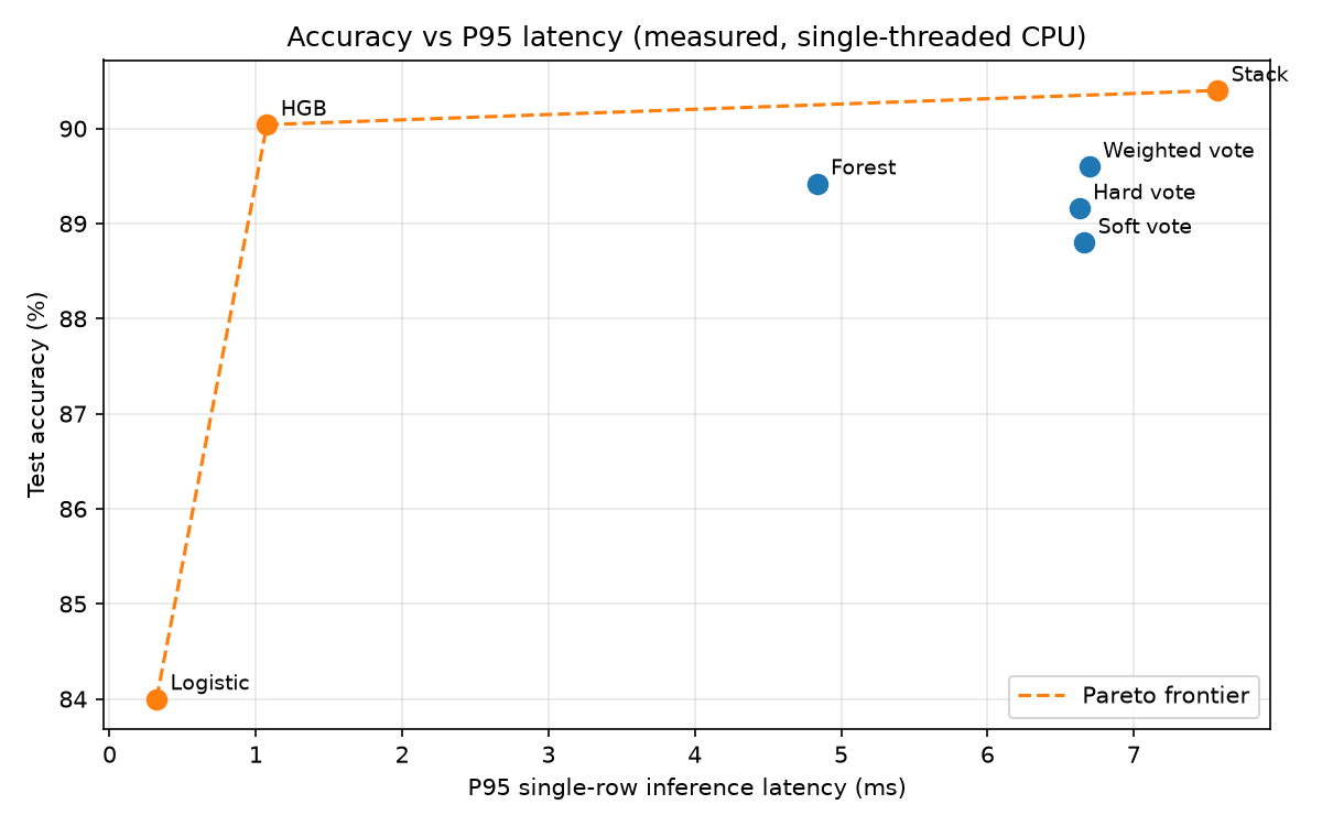
Test accuracy versus P95 inference latency, measured in the run above. Up and to the left is better; the dashed line is the Pareto frontier.
The results illustrate a common outcome: the most accurate ensemble is not automatically the best system.
In this experiment, the strongest individual model is histogram-based gradient boosting.
Its accuracy is 90.04%, with P95 inference latency of approximately 1.08 milliseconds.
Stacking improves accuracy to 90.40%, but its P95 latency increases to approximately 7.57 milliseconds.
The difference is:
-
Accuracy improvement: +0.36 percentage points
-
Additional P95 latency: approximately 6.50 milliseconds
-
P95 latency multiplier: approximately 7.0×
Whether that trade-off is worthwhile depends entirely on the application.
For a batch analytics job, the increase may be inconsequential. For a service handling a large volume of latency-sensitive requests, it may not be justified.
Why didn’t voting win?
The voting models all underperformed the best individual model.
This is an important empirical result, not a failed experiment.
Voting assumes that combining several predictions will provide better decisions. But adding a weaker model can dilute a stronger model’s useful signal.
The linear classifier, for example, has considerably lower accuracy than the two tree-based models. Giving it the same voting influence can hurt rather than help.
Weighted voting reduces that influence, which explains why it performs somewhat better than the unweighted version in this particular experiment.
But the weighting strategy still doesn’t surpass the strongest individual baseline.
Stacking achieves a small improvement by learning how to use the base model predictions instead of assigning them equal or manually chosen weights.
This suggests an obvious next question: do we actually need all three models?
5. Reduce the ensemble before optimizing it
Adding more models is easy. Removing unnecessary models is often where the real engineering value appears.
Our first experiment suggests that logistic regression contributes relatively little to this particular ensemble. Let’s evaluate a simpler combination containing only random forest and histogram-based gradient boosting.
Append the following code to the benchmark script:
# Combine only the two tree-based models.
lean_ensemble = VotingClassifier(
    estimators=[
        ("forest", clone(base["Forest"])),
        ("hgb", clone(base["HGB"])),
    ],
    voting="soft",
    n_jobs=1,
)

lean_ensemble.fit(X_train, y_train)

lean_accuracy = accuracy_score(
    y_test,
    lean_ensemble.predict(X_test),
)

lean_p50, lean_p95, lean_batch = benchmark(
    lean_ensemble,
    X_test,
)

print("\nTwo-model soft voting:")
print(f"Accuracy: {lean_accuracy:.4f}")
print(f"P50 latency: {lean_p50:.3f} ms")
print(f"P95 latency: {lean_p95:.3f} ms")
print(f"Batch latency: {lean_batch:.3f} ms")
In a local run, this two-model combination achieved:
-
Accuracy: 90.13%
-
P50 latency: approximately 6.24 ms
-
P95 latency: approximately 6.84 ms
It recovered part of stacking’s gain (90.13% versus 90.40%) with one model less and a slightly lower P95, but it still cost several times the latency of histogram boosting alone.
We should not conclude that two-model voting is universally better or worse than stacking. Differences of a few tenths of a percentage point are specific to this dataset and split, and the latency gap could vary between benchmark runs.
Nevertheless, this is an excellent reason to investigate smaller ensembles before adding more sophisticated combination layers.
Examine the Pareto frontier
A model is Pareto-dominated when another model has both:
-
Equal or better accuracy.
-
Equal or lower latency.
At least one comparison must be strictly better.
Under these criteria, dominated models offer no advantage on the measured dimensions.
We can calculate the accuracy–latency frontier directly from the benchmark results.
Append this code:
# Identify non-dominated models using accuracy and P95 latency.
pareto_models = []

for name, values in results.items():
    accuracy = values[0]
    p95 = values[3]

    dominated = False

    for other_name, other_values in results.items():
        if name == other_name:
            continue

        other_accuracy = other_values[0]
        other_p95 = other_values[3]

        at_least_as_good = (
            other_accuracy >= accuracy
            and other_p95 <= p95
        )

        strictly_better = (
            other_accuracy > accuracy
            or other_p95 < p95
        )

        if at_least_as_good and strictly_better:
            dominated = True
            break

    if not dominated:
        pareto_models.append(name)

print("\nPareto-efficient models:")

for name in sorted(
    pareto_models,
    key=lambda n: results[n][3],
):
    accuracy, _, _, p95, _ = results[name]
    print(
        f"{name}: "
        f"accuracy={accuracy:.4f}, "
        f"p95={p95:.3f} ms"
    )
Using the original seven models and our measured results, the Pareto frontier contains:
-
Logistic regression: extremely fast, but less accurate.
-
Histogram-based gradient boosting: strong accuracy with low latency.
-
Stacking: slightly higher accuracy at considerably higher latency.
The remaining models are dominated by at least one alternative.
This is a useful way to narrow a deployment decision. Instead of comparing every experimental model, focus on candidates that offer a meaningful trade-off.
The frontier may change when memory usage, calibration, throughput, infrastructure cost, or model maintenance are included.
6. How stacking avoids a common form of data leakage
Stacking is more complicated than voting because it introduces a second learned model.
Consider a straightforward but flawed stacking procedure:
-
Train three models on a training dataset.
-
Generate predictions from those models on the same training dataset.
-
Use those predictions to train another model.
-
Evaluate the combined system on unseen data.
The problem occurs in the second step.
The base models may have memorized details of their training examples. Their predictions on those examples are therefore not representative of predictions on unseen observations.
A meta-model trained on these overly optimistic predictions can learn misleading relationships.
This is a form of training-data leakage between the base layer and the meta-model.
The correct approach: out-of-fold predictions
The solution is to train the meta-model on predictions generated for samples that were not used to fit the corresponding base models.
For four-fold stacking:
| Fold | Base models trained on | Predictions generated for |
|---|---|---|
| 1 | Folds 2, 3, 4 | Fold 1 |
| 2 | Folds 1, 3, 4 | Fold 2 |
| 3 | Folds 1, 2, 4 | Fold 3 |
| 4 | Folds 1, 2, 3 | Fold 4 |
Each training example receives predictions from base models that did not train on that example.
These out-of-fold predictions become the training features for the meta-model.
Afterward, the base estimators are fitted on the complete training dataset for deployment.
At inference time:
-
Each fully fitted base model predicts the incoming example.
-
The predictions form a small feature vector.
-
The trained meta-model processes that vector.
-
The meta-model returns the final prediction.
This architecture distinguishes stacking from ordinary voting.
What scikit-learn does automatically
The StackingClassifier implementation handles the necessary out-of-fold training internally.
Its cross-validation parameter determines how the meta-model’s training features are generated.
For binary classification, when the stack uses predicted probabilities, scikit-learn drops one of the two probability columns from each base estimator. The probabilities sum to one, so retaining both would introduce perfect collinearity.
In our example, the meta-model learns from three probability-derived features, one for each base estimator.
Also note that we disabled feature passthrough. The meta-model does not receive the original 20 features, only the base models’ predictions.
Turning passthrough on is a valid additional experiment, but it changes the modeling problem. It gives the final estimator access to the original inputs as well as the predictions.
Why training is more expensive
Four-fold stacking requires additional fitting work to produce out-of-fold predictions.
For three base models, this means multiple cross-validation fits, followed by fitting the base models on the complete training dataset and training the final estimator.
That explains why stacking has a substantially higher training time in our benchmark.
Crucially, cross-validation multiplies training work, not inference work.
At inference time, the stack uses the fully fitted base models once each, followed by one meta-model prediction. It does not execute every model fitted during cross-validation.
This distinction matters when estimating production cost.
For further implementation details, consult the official scikit-learn ensemble documentation.
7. Why soft voting sometimes loses to hard voting
It is tempting to assume that probability-based voting is automatically superior because it uses more information.
That assumption overlooks probability calibration.
Consider two models:
-
Model A predicts a probability of 0.95 when it is moderately confident.
-
Model B predicts a probability of 0.65 for examples where it has a similar empirical success rate.
The first model may dominate a probability average even when its predictions are less reliable.
A well-calibrated classifier should produce positive outcomes approximately 70% of the time among examples assigned a probability near 0.70.
Accuracy alone does not establish good calibration.
Measure probability quality
For probability-based ensembles, useful evaluation metrics include:
-
Log loss: Penalizes incorrect probability estimates, particularly overconfident mistakes.
-
Brier score: Measures the squared difference between predicted probabilities and binary outcomes.
-
Calibration curves: Compare predicted probabilities against observed positive frequencies.
These complement classification accuracy.
For example, two models may achieve exactly the same accuracy while one produces probabilities that are substantially more useful for ranking, risk estimation, or threshold selection.
Calibrate before combining
If base models provide poorly calibrated probabilities, probability calibration may improve the reliability of soft voting.
Scikit-learn provides CalibratedClassifierCV for this purpose.
However, calibration should be learned using appropriately separated data or cross-validation. Fitting a calibration model using the final evaluation set would introduce leakage.
Calibration also adds training complexity and can affect inference latency.
The right order is therefore:
-
Measure base-model accuracy and probability quality.
-
Evaluate calibration on development data.
-
Reassess voting weights using validation data.
-
Compare the calibrated ensemble against the original baseline.
-
Confirm the result on a separate, untouched test set.
Do not add calibration automatically merely because an ensemble uses probabilities.
8. Measure the latency your application actually experiences
Our benchmark measures the Python prediction calls directly.
That is useful for comparing algorithmic overhead, but it is not equivalent to measuring a complete production service.
A deployed prediction endpoint can include:
-
Request parsing and validation.
-
Data retrieval and feature generation.
-
Serialization and deserialization.
-
Model execution.
-
Ensemble combination.
-
Network communication.
-
Logging, tracing, and monitoring.
-
Queueing during bursts of traffic.
For many applications, these additional stages dominate total response time.
P50 versus P95 versus P99
Median latency describes a typical request.
P95 latency means approximately 95% of observed requests completed within that time.
P99 focuses on the slowest 1% of observed requests.
For interactive systems, tail latency can be more important than average latency because slow responses may directly affect users.
Our experiment uses 200 timed single-sample predictions per model, which is sufficient for a small comparative demonstration but not for a reliable production tail-latency assessment.
A production benchmark should use substantially more requests, repeat measurements across runs, and include representative concurrency.
Batch size changes the economics
A model may be inefficient when called once for every sample but considerably more efficient when processing a batch.
The reasons include:
-
Less Python invocation overhead per sample.
-
More efficient vectorized computation.
-
Better opportunities for memory reuse.
-
Amortization of some fixed prediction costs.
Our script measures both individual requests and batches of 256 examples to expose this difference.
Batch throughput can be estimated as:
Throughput = batch size / batch execution time in seconds
For example, a batch of 256 examples processed in 8 milliseconds corresponds to a batch-only processing rate of 32,000 examples per second.
That figure is not necessarily the sustainable throughput of a deployed endpoint. It excludes data acquisition, network overhead, queueing, and other serving costs.
It is also important not to confuse batch efficiency with interactive latency.
A large batch can improve throughput while forcing early-arriving requests to wait for the batch to fill.
Parallel inference is not free
One way to reduce ensemble latency is to execute base models concurrently.
This approach can help when model execution times are substantial and resources are available.
But increasing parallelism does not guarantee better performance.
Common problems include:
-
CPU oversubscription.
-
Memory bandwidth contention.
-
Higher peak memory usage.
-
Scheduling overhead for small predictions.
-
Increased infrastructure consumption.
-
Interference between simultaneous requests.
The n_jobs option in relevant scikit-learn ensemble implementations controls parallelism for fitting base estimators. It should not be interpreted as a guarantee that prediction calls will run concurrently.
If prediction-time parallelism is required, benchmark an explicit serving architecture that provides it.
For CPU-bound single-row inference, running several separate prediction workers may even be slower than a sequential implementation.
9. When is the additional accuracy worth the latency?
The most interesting number from our benchmark is not 90.40%.
It is the difference between 90.40% and 90.04%.
On a test set containing 1,125 samples, the stacking model correctly classified 1,017 examples, compared with 1,013 for histogram-based gradient boosting.
That represents just four additional correct predictions in this particular test.
This small difference raises two questions.
First, is the improvement repeatable?
Second, are those additional correct predictions valuable enough to justify the extra work?
Statistical reliability comes first
A difference of four correct predictions on one test set provides limited evidence of generalizable superiority.
We should examine:
-
Performance across multiple random seeds and data splits.
-
Paired uncertainty estimates, such as bootstrapped confidence intervals for the accuracy difference.
-
Accuracy on genuinely new data.
-
Stability across different groups and operating conditions.
-
Performance when the distribution of incoming data changes.
If a team tests dozens of ensemble configurations against the same holdout and chooses the best result, that holdout gradually becomes a model-selection dataset.
A better evaluation process uses separate training, validation, and final test data, or appropriate nested cross-validation.
For temporal data, such as real e-commerce transactions, evaluation should often preserve time order rather than relying entirely on random splits.
In our tutorial, the test set serves as a controlled exploratory comparison. A production decision would require fresh evaluation after model selection.
Business value matters more than percentage points
Accuracy treats every correct classification as equally valuable.
Real decisions rarely work that way.
In an order-review system, incorrectly approving a problematic transaction may be more expensive than unnecessarily sending a harmless transaction for review.
A model that improves overall accuracy could still increase business cost if it makes more mistakes in the expensive category.
Consequently, evaluate:
-
False-positive and false-negative rates.
-
Precision and recall at the intended decision threshold.
-
Operational costs of different errors.
-
Predicted probability quality.
-
Latency and infrastructure cost.
-
The number of decisions affected by the model change.
A useful conceptual decision rule is:
Net benefit = value of improved decisions − added computation cost − latency-related business cost − operational complexity
All terms should be estimated for the intended workload rather than inferred from accuracy alone.
A practical deployment decision matrix
| Situation | Likely recommendation |
|---|---|
| Strict real-time latency budget | Prefer the strongest single model that meets the budget |
| Offline batch predictions | Consider voting or stacking when quality gains are reliable |
| Expensive prediction mistakes | Evaluate ensembles using error-specific business costs |
| Models with highly correlated errors | Focus on diversity or improve individual models |
| Large accuracy improvements from a small ensemble | Strong candidate for deployment |
| Tiny gains from many expensive models | Prefer simpler alternatives unless business value is proven |
| Unstable improvement across evaluation periods | Collect stronger evidence before deployment |
The latency budget should be assessed against the complete serving system, not just the model’s prediction call.
10. Cherry on the cake: the Netflix Prize ensemble that never made it into production
One of the most memorable examples of this trade-off comes from the Netflix Prize.
In 2006, Netflix launched a competition offering $1 million for a recommendation algorithm that improved prediction of movie ratings by at least 10% relative to its Cinematch baseline, measured using root mean squared error.
In 2009, the team BellKor’s Pragmatic Chaos won the Grand Prize with a sophisticated combination of recommendation models.
The winning approach represented years of experimentation and combined hundreds of predictive models.
Yet Netflix did not deploy the complete Grand Prize ensemble.
In an April 6, 2012 engineering article, Netflix explained that it had evaluated some of the additional methods offline, but the measured accuracy improvements did not justify the engineering effort required for production deployment.
The company had also shifted its personalization priorities as its business evolved from DVD rentals toward streaming.
There is an important nuance: Netflix did deploy two underlying approaches originating from an earlier Progress Prize solution, after adapting them for production-scale data. It was the full Grand Prize ensemble that was not adopted.
So it would be inaccurate to conclude that Netflix simply found the winning code too slow. The documented problem was broader: the incremental benefit did not justify the operational engineering effort, especially as the business objective evolved.
The lesson remains highly relevant.
A competition rewards performance against a specified evaluation metric. A production system must also satisfy operational requirements, scalability constraints, maintenance needs, and changing product priorities.
The best benchmark model and the best deployable model are not necessarily the same.
Sources: Netflix Technology Blog — Netflix Recommendations: Beyond the 5 Stars (Part 1), Wired’s reporting on the production decision.
11. A production checklist for inference-time ensembles
Before deploying a voting or stacking system, evaluate four areas.
Predictive performance
-
Compare against the strongest individual model, not merely the weakest baseline.
-
Measure improvements on genuinely unseen data.
-
Validate probability calibration where applicable.
-
Examine error overlap and error-specific costs.
-
Repeat experiments to establish whether improvements are stable.
Inference performance
-
Measure single-request and batch latency.
-
Report P50, P95, and P99 under representative load.
-
Include preprocessing and network overhead.
-
Measure peak memory use and CPU utilization.
-
Test concurrent requests rather than only isolated calls.
Operational reliability
-
Version each base model and the ensemble combination logic.
-
Ensure preprocessing is consistent across training and inference.
-
Monitor individual model outputs as well as the final output.
-
Define what happens if one model becomes unavailable.
-
Provide a rollback path to a reliable single-model baseline.
A partial ensemble failure deserves particular attention. Silently replacing a missing model with a default prediction changes the ensemble’s behavior and may invalidate its probability interpretation.
Fallback behavior should be explicitly designed, tested, and monitored.
Model lifecycle
-
Automate reproducible training and evaluation.
-
Keep cross-validation and ensemble-weight selection separate from final testing.
-
Track the additional time needed to retrain the ensemble.
-
Monitor changes in data distribution and error patterns.
-
Reassess whether every model in the ensemble still contributes value.
An ensemble that is useful today may become unnecessarily expensive after its strongest individual model improves.
12. Key lessons from the experiment
Our results support several practical conclusions.
First, ensembles are not guaranteed to outperform their individual components. Both hard voting and unweighted soft voting performed worse than the strongest base model in this experiment.
Second, learned combinations can outperform simple aggregation. Stacking achieved the highest accuracy among our original seven configurations, although the improvement was small.
Third, adding models creates measurable costs. The stacking ensemble delivered an accuracy increase of approximately 0.36 percentage points while increasing measured single-request P95 latency by a factor of roughly seven relative to the strongest single model.
Fourth, simpler combinations deserve serious consideration. A two-model voting ensemble matched stacking accuracy on our test set, demonstrating why model pruning is worth evaluating before building a more complex serving architecture.
Finally, accuracy is only one dimension of model quality. Latency, throughput, calibration, operating costs, reliability, and maintainability all influence whether an ensemble should be deployed.
The goal is not to build the largest possible collection of models. It is to find the smallest, most reliable system that satisfies the application’s predictive and operational requirements.
13. Your next experiment
Run the benchmark on your own machine, then modify the ensemble one component at a time.
A useful exercise is to compare three candidates: the best individual model, the two-model voting ensemble, and the stacking ensemble. Repeat the evaluation across several random seeds, measure latency under concurrent requests, and determine which models remain on the accuracy–latency Pareto frontier.
Then apply the same methodology to an appropriate real-world dataset, such as retail orders, equipment sensor readings, or server telemetry.
Your challenge: Find an ensemble that delivers a statistically credible accuracy improvement while remaining within a strict P95 inference-latency budget.
If no ensemble meets that requirement, deploy the simpler model. Choosing not to ensemble can be just as important an engineering decision as choosing how to ensemble.