
LEARN · GRADIENT BOOSTING WITH XGBOOST
The mental model: regularize both the leaf score and the split
XGBoost does not regularize a tree in quite the same way that ridge regression or Lasso regularizes a linear model. A standard tree booster does not have one coefficient per input feature. Instead, it assigns prediction weights to leaves, decides which splits deserve to exist, and adds successive trees to an ensemble.
That creates several distinct ways to control complexity:
-
reg_lambdashrinks leaf weights through L2 regularization. -
reg_alphaapplies L1 regularization, which can drive leaf weights exactly to zero. -
gammarequires a split to achieve sufficient loss reduction. -
min_child_weightrequires each proposed child to have enough accumulated Hessian weight. -
max_depthandmax_leaveslimit tree structure. -
subsampleandcolsample_bytreeintroduce randomness into tree construction. -
Early stopping limits the number of boosting rounds retained for prediction.
-
Monotonic and interaction constraints restrict which relationships the model can represent.
These mechanisms overlap, but they are not interchangeable. A deep tree with conservative leaf weights can generalize better than a shallow tree whose leaves make aggressive, poorly supported corrections.
The distinction matters when training error continues to fall while validation error stops improving. The objective is not to make training error as large as possible or to produce the smallest possible trees. It is to retain structures that capture reproducible signal while suppressing corrections that primarily explain noise.
This tutorial uses XGBoost 3.4.1 (the current PyPI wheel) and a synthetic, non-medical regression dataset. The experiments separate training, validation, and test data, measure tree structure alongside predictive error, and generate their results directly from the fitted models.
The objective behind the controls
For a tree added during boosting, XGBoost uses a second-order approximation of the loss together with a complexity penalty. The regularized objective can be expressed schematically as:
Objective ≈ data loss + γT + (λ/2) Σⱼ wⱼ² + α Σⱼ |wⱼ|
Here:
-
Tis the number of leaves in the tree. -
wⱼis the prediction weight assigned to leaf j. -
λis the L2 penalty, exposed asreg_lambda. -
αis the L1 penalty, exposed asreg_alpha. -
γis the per-leaf complexity penalty, exposed asgamma.
The expression captures two different decisions: how large a prediction correction should be, and whether a more complex tree structure is worth creating.
During boosting, XGBoost calculates gradients and Hessians from the current predictions. For a candidate leaf, let G be the sum of the gradients of its training instances and H be the sum of their Hessians.
With L2 regularization and no L1 penalty, the optimal leaf weight before learning-rate shrinkage is:
w* = −G / (H + λ)
This formula is the foundation for understanding the four principal controls.
The numerator represents the accumulated direction and strength of the proposed correction. The denominator combines the curvature supported by the observations with the L2 penalty.
Increasing reg_lambda reduces the magnitude of the correction. Increasing reg_alpha can eliminate the correction altogether. Increasing gamma raises the hurdle a split must clear, while increasing min_child_weight prevents children with insufficient Hessian support from being created.
For the complete parameter definitions, see the official XGBoost parameter reference.
1. reg_lambda: shrink leaf weights without necessarily removing leaves
L2 regularization is a useful first control because it reduces the influence of individual leaves while allowing the model to retain a relatively expressive structure.
Consider a hypothetical leaf with G = −24 and H = 12. Ignoring the learning rate, its optimal weight under different L2 penalties is:
reg_lambda |
Calculation | Leaf weight |
|---|---|---|
| 0 | 24 / 12 | 2.00 |
| 12 | 24 / 24 | 1.00 |
| 36 | 24 / 48 | 0.50 |
The direction of the update remains the same, but its magnitude decreases as the penalty increases. The leaf can still contribute to the ensemble; its correction simply becomes more conservative.
Why it helps
Deep trees can isolate small groups of observations with unusually large residuals. Some of those residuals represent genuine patterns, but others are random deviations that will not recur in new data.
Without sufficient regularization, the model can assign large weights to these groups, substantially reducing training error without producing a comparable improvement in validation performance.
A positive L2 penalty discourages extreme leaf values. It also affects split-gain calculations, so increasing reg_lambda can indirectly change the tree structure by making some splits less attractive.
What to measure
Inspect three quantities together:
-
Training RMSE at the best validation round.
-
Validation RMSE at that same round.
-
Mean number of leaves per tree.
If validation RMSE improves while training RMSE rises modestly, the model is giving up some sample-specific fit in exchange for better generalization. If tree sizes also decline, the penalty is influencing structure as well as leaf weights.
If both training and validation error deteriorate substantially, the penalty may be suppressing genuine signal.
2. reg_alpha: make weak leaf corrections disappear
L1 regularization is more selective than L2 regularization. Instead of merely shrinking every correction, it can set weak leaf weights exactly to zero.
With gradient sum G, Hessian sum H, L1 penalty α, and L2 penalty λ, the optimal leaf weight is:
w* = −sign(G) × max(|G| − α, 0) / (H + λ)
The operation max(|G| − α, 0) is a soft-thresholding function.
When the absolute gradient sum does not exceed the L1 penalty, the optimal weight is zero. Otherwise, the penalty subtracts α from the gradient magnitude before calculating the weight.
For example, with G = −4, H = 10, and λ = 0:
reg_alpha |
Leaf weight |
|---|---|
| 0 | 0.40 |
| 2 | 0.20 |
| 4 | 0.00 |
| 6 | 0.00 |
The difference from L2 is important: L1 can eliminate a weak correction rather than merely reducing its magnitude.
A zero-weight leaf does not necessarily mean that its structural node is physically removed from the tree. The penalty acts directly on leaf scores, although it can also influence whether candidate splits are accepted.
Use reg_alpha when weak corrections appear unnecessary, particularly in models with noisy features and many small partitions. Compare validation error and leaf counts rather than assuming that a sparser set of weights must produce better predictions.
3. gamma: require every split to earn its place
gamma, also called min_split_loss, controls the minimum loss reduction required for a split to be accepted.
With L1 regularization disabled, a simplified split-gain expression is:
Gain = ½ [Gₗ² / (Hₗ + λ) + Gᵣ² / (Hᵣ + λ) − G² / (H + λ)] − γ
The left and right subscripts describe the proposed children. The unsubscripted quantities describe the parent.
The terms inside the brackets compare the quality of the two children with the quality of the parent. The difference estimates the improvement obtained by splitting, before subtracting the complexity penalty.
When L1 regularization is enabled, the gain calculation also incorporates thresholded gradient sums.
Suppose a candidate split provides a gain of 3 before subtracting gamma.
-
With
gamma = 0, the split can be accepted. -
With
gamma = 1, the split can still be accepted. -
With
gamma = 5, the split is rejected.
A binary split adds another leaf, so the per-leaf complexity penalty raises the required gain for further partitioning.
This can reduce tree sizes dramatically. However, the numerical scale is specific to the training objective and data. A value of 5 is not universally conservative, and a value of 1 is not universally small.
Use gamma when the model creates many marginal splits that add complexity without sufficient improvement in the regularized objective. If the trees shrink but validation error increases, the penalty is removing useful structure as well as noise.
One subtle point: a tree with no accepted splits can still contain a single leaf with a nonzero prediction weight. Refusing to split does not necessarily mean refusing to make a prediction correction.
4. min_child_weight: demand enough Hessian mass
min_child_weight controls the minimum sum of instance Hessians required in a child.
It is not universally a minimum row count.
For unweighted squared-error regression with the standard reg:squarederror objective, each observation contributes a Hessian of 1. In that specific setting, the accumulated Hessian is equivalent to the number of observations in the child.
For other objectives, Hessians can vary. In logistic regression, for example, the Hessian depends on the predicted probability. A child can contain many observations yet have relatively little accumulated Hessian weight.
This makes min_child_weight a measure of optimization support rather than a universal sample-count threshold.
Why it helps with noisy leaves
A deep tree can repeatedly partition the data until it isolates tiny groups with unusually large residuals. Those groups can provide attractive-looking corrections even when their patterns are unstable.
Increasing min_child_weight blocks splits that would create children without sufficient Hessian mass. It is therefore a direct control when the model depends too heavily on small, weakly supported partitions.
Its role differs from that of gamma:
-
gammaasks whether a split delivers sufficient loss reduction. -
min_child_weightasks whether the proposed children have sufficient Hessian support.
A split can have attractive gain and still be inadmissible because one of its children lacks the required Hessian mass.
5. Measure the effects with controlled sweeps
Parameter explanations describe what the controls are intended to do. An experiment reveals whether those effects improve the task at hand.
The following experiment uses 8,000 synthetic observations with 18 numeric features. The target contains nonlinear effects, interactions, a threshold effect, and random noise. This creates both genuine patterns and opportunities for the model to overfit.
The data is split into three independent partitions:
-
60% training data for fitting model parameters.
-
20% validation data for comparing settings and selecting boosting rounds.
-
20% test data reserved for one final evaluation.
The test set is not used during parameter sweeps, early stopping, or the shallow-versus-deep comparison.
Pin the environment
The latest XGBoost wheel on PyPI is 3.4.1, which is what this lesson pins. A newer 3.4.2 source tag exists; if you prefer it, follow the official build instructions and change the pin in the script. The parameters used here behave the same in both.
Create a requirements.txt file with these exact Python dependency versions:
numpy==2.5.4
pandas==3.0.6
scikit-learn==1.9.1
scipy==1.18.1
matplotlib==3.11.2
xgboost==3.4.1
Create the environment and install the pinned dependencies:
python3 -m venv .venv
source .venv/bin/activate
python -m pip install -r requirements.txt
The experiment checks the installed package versions before training. It prints the measured results and writes them to CSV files, so the reported RMSE, best rounds, and leaf counts all come from the same execution rather than from a manually transcribed table produced under a different release.
Run the experiment
Save the following as regularization_experiment.py in the directory containing requirements.txt.
import json
import platform

import matplotlib
import matplotlib.pyplot as plt
import numpy as np
import pandas as pd
import sklearn
import xgboost as xgb

from sklearn.model_selection import train_test_split
from xgboost import XGBRegressor


EXPECTED_VERSIONS = {
    "xgboost": "3.4.1",
    "numpy": "2.5.4",
    "pandas": "3.0.6",
    "scikit-learn": "1.9.1",
    "scipy": "1.18.1",
    "matplotlib": "3.11.2",
}

ACTUAL_VERSIONS = {
    "xgboost": xgb.__version__,
    "numpy": np.__version__,
    "pandas": pd.__version__,
    "scikit-learn": sklearn.__version__,
    "scipy": __import__("scipy").__version__,
    "matplotlib": matplotlib.__version__,
}

print("Python:", platform.python_version())
print("Package versions:", ACTUAL_VERSIONS)

if ACTUAL_VERSIONS != EXPECTED_VERSIONS:
    raise RuntimeError(
        "Package versions differ from the pinned environment. "
        f"Expected {EXPECTED_VERSIONS}, got {ACTUAL_VERSIONS}"
    )


# Generate a reproducible nonlinear regression dataset.
rng = np.random.default_rng(20261016)

X = rng.normal(size=(8000, 18)).astype(np.float32)

y = (
    2.5 * np.sin(1.6 * X[:, 0])
    + 0.9 * (X[:, 1] ** 2 - 1.0)
    + 1.8 * X[:, 2] * X[:, 3]
    + 1.4 * (X[:, 4] > 0.35)
    + 1.1 * np.maximum(X[:, 5], 0)
    + 0.8 * X[:, 6] * X[:, 7]
    + 0.5 * X[:, 0] * X[:, 4]
    + rng.normal(0, 1.1, size=len(X))
).astype(np.float32)


# Reserve the test set before any model selection.
X_dev, X_test, y_dev, y_test = train_test_split(
    X,
    y,
    test_size=0.20,
    random_state=71,
)

X_train, X_valid, y_train, y_valid = train_test_split(
    X_dev,
    y_dev,
    test_size=0.25,
    random_state=17,
)

print(
    "Rows:",
    {
        "train": len(y_train),
        "validation": len(y_valid),
        "test": len(y_test),
    },
)


def count_leaves(node):
    """Count terminal nodes in a JSON tree."""
    if "leaf" in node:
        return 1

    return sum(
        count_leaves(child)
        for child in node["children"]
    )


def mean_leaves_at_round(model, n_rounds):
    """Measure mean leaves over the selected tree prefix."""
    trees = model.get_booster().get_dump(
        dump_format="json"
    )[:n_rounds]

    leaves = [
        count_leaves(json.loads(tree))
        for tree in trees
    ]

    return float(np.mean(leaves))


def fit_and_measure(
    params,
    n_estimators,
    learning_rate,
    early_stopping_rounds,
):
    """Fit on training data and select rounds using validation."""
    model = XGBRegressor(
        objective="reg:squarederror",
        eval_metric="rmse",
        tree_method="hist",
        n_estimators=n_estimators,
        learning_rate=learning_rate,
        n_jobs=4,
        random_state=42,
        early_stopping_rounds=early_stopping_rounds,
        **params,
    )

    model.fit(
        X_train,
        y_train,
        eval_set=[
            (X_train, y_train),
            (X_valid, y_valid),
        ],
        verbose=False,
    )

    evaluation = model.evals_result()

    train_curve = np.asarray(
        evaluation["validation_0"]["rmse"]
    )
    valid_curve = np.asarray(
        evaluation["validation_1"]["rmse"]
    )

    best_index = int(np.argmin(valid_curve))
    best_round = best_index + 1

    return {
        "model": model,
        "train_curve": train_curve,
        "valid_curve": valid_curve,
        "best_index": best_index,
        "best_round": best_round,
        "train_rmse": float(train_curve[best_index]),
        "validation_rmse": float(valid_curve[best_index]),
        "mean_leaves": mean_leaves_at_round(
            model,
            best_round,
        ),
    }


# Sweep one primary regularization parameter at a time.
baseline = {
    "reg_lambda": 1.0,
    "reg_alpha": 0.0,
    "gamma": 0.0,
    "min_child_weight": 1.0,
}

sweeps = {
    "reg_lambda": [0, 1, 10, 100],
    "reg_alpha": [0, 1, 5],
    "gamma": [0, 1, 10, 100],
    "min_child_weight": [1, 10, 50, 100],
}

sweep_rows = []
sweep_curves = {}

for parameter, values in sweeps.items():
    for value in values:
        params = baseline.copy()
        params[parameter] = value

        measured = fit_and_measure(
            params=params,
            n_estimators=600,
            learning_rate=0.08,
            early_stopping_rounds=40,
        )

        sweep_curves[(parameter, value)] = (
            measured["train_curve"],
            measured["valid_curve"],
        )

        sweep_rows.append({
            "parameter": parameter,
            "value": value,
            "best_round": measured["best_round"],
            "train_rmse": measured["train_rmse"],
            "validation_rmse": measured["validation_rmse"],
            "mean_leaves": measured["mean_leaves"],
        })

sweep_results = pd.DataFrame(sweep_rows)

sweep_results.to_csv(
    "regularization_sweep.csv",
    index=False,
)

print("\nIndividual parameter sweeps:")
print(
    sweep_results.round(4).to_string(index=False)
)


# Plot training and validation curves for the lowest
# and highest tested value of each parameter.
fig, axes = plt.subplots(
    2,
    2,
    figsize=(13, 8),
    constrained_layout=True,
)

for ax, (parameter, values) in zip(
    axes.flat,
    sweeps.items(),
):
    for value in [values[0], values[-1]]:
        train_curve, valid_curve = sweep_curves[
            (parameter, value)
        ]

        rounds = np.arange(1, len(train_curve) + 1)

        ax.plot(
            rounds,
            train_curve,
            label=f"{value}: train",
        )

        ax.plot(
            rounds,
            valid_curve,
            linestyle="--",
            label=f"{value}: validation",
        )

    ax.set_title(parameter)
    ax.set_xlabel("Boosting round")
    ax.set_ylabel("RMSE")
    ax.legend(fontsize=8)

fig.savefig(
    "regularization_curves.png",
    dpi=160,
)

plt.show()


# Compare a shallow, unregularized model with a deeper,
# explicitly regularized model.
comparison_configs = {
    "shallow_unregularized": {
        "max_depth": 2,
        "reg_lambda": 0.0,
        "reg_alpha": 0.0,
        "gamma": 0.0,
        "min_child_weight": 1.0,
        "subsample": 1.0,
        "colsample_bytree": 1.0,
    },
    "deep_regularized": {
        "max_depth": 8,
        "reg_lambda": 10.0,
        "reg_alpha": 1.0,
        "gamma": 0.0,
        "min_child_weight": 50.0,
        "subsample": 0.8,
        "colsample_bytree": 0.8,
    },
}

comparison_rows = []
comparison_curves = {}

for name, params in comparison_configs.items():
    measured = fit_and_measure(
        params=params,
        n_estimators=1200,
        learning_rate=0.05,
        early_stopping_rounds=50,
    )

    comparison_curves[name] = (
        measured["train_curve"],
        measured["valid_curve"],
    )

    comparison_rows.append({
        "model": name,
        **params,
        "best_round": measured["best_round"],
        "train_rmse": measured["train_rmse"],
        "validation_rmse": measured["validation_rmse"],
        "mean_leaves": measured["mean_leaves"],
    })

comparison_results = (
    pd.DataFrame(comparison_rows)
    .sort_values("validation_rmse")
    .reset_index(drop=True)
)

comparison_results.to_csv(
    "depth_comparison.csv",
    index=False,
)

print("\nShallow-versus-deep comparison:")
print(
    comparison_results.round(4).to_string(index=False)
)


fig, ax = plt.subplots(figsize=(10, 5))

for name, (train_curve, valid_curve) in comparison_curves.items():
    train_rounds = np.arange(1, len(train_curve) + 1)
    valid_rounds = np.arange(1, len(valid_curve) + 1)

    ax.plot(
        train_rounds,
        train_curve,
        label=f"{name}: train",
    )

    ax.plot(
        valid_rounds,
        valid_curve,
        linestyle="--",
        label=f"{name}: validation",
    )

ax.set_xlabel("Boosting round")
ax.set_ylabel("RMSE")
ax.legend()
fig.tight_layout()
fig.savefig("depth_comparison_curves.png", dpi=160)
plt.show()


# Select the winner using validation RMSE only.
winner = comparison_results.iloc[0]
winner_name = str(winner["model"])
winner_rounds = int(winner["best_round"])
winner_params = comparison_configs[winner_name]


# Refit the selected configuration on all development data.
# The test set has not been used during fitting or selection.
X_development = np.concatenate(
    [X_train, X_valid],
    axis=0,
)
y_development = np.concatenate(
    [y_train, y_valid],
    axis=0,
)

final_model = XGBRegressor(
    objective="reg:squarederror",
    eval_metric="rmse",
    tree_method="hist",
    n_estimators=winner_rounds,
    learning_rate=0.05,
    n_jobs=4,
    random_state=42,
    **winner_params,
)

final_model.fit(
    X_development,
    y_development,
    verbose=False,
)


# Evaluate the untouched test set once, after model selection.
test_predictions = final_model.predict(X_test)

test_rmse = float(
    np.sqrt(
        np.mean(
            (y_test - test_predictions) ** 2
        )
    )
)

print("\nFinal evaluation:")
print("Selected configuration:", winner_name)
print("Selected boosting rounds:", winner_rounds)
print(f"Untouched test RMSE: {test_rmse:.4f}")
Run the script:
python regularization_experiment.py
It generates four artifacts:
-
regularization_sweep.csv— measured RMSE, best boosting round, and mean leaves for each parameter setting. -
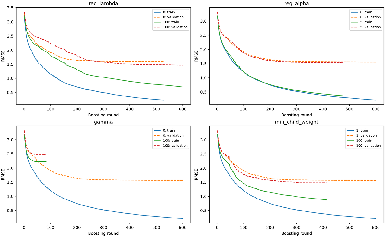
regularization_curves.png— training and validation curves for the low and high settings of each parameter. -
depth_comparison.csv— measured results for the shallow and deep configurations. -
depth_comparison_curves.png— learning curves for those two configurations.
The test RMSE is printed only after the comparison has selected a configuration and the final model has been refitted on the combined training and validation data.
How to interpret the measured results
The experiment records training RMSE and validation RMSE at the best validation round, rather than comparing arbitrary points on curves that may have stopped at different times.
It also measures mean leaves per tree over the same selected tree prefix. This is more informative than assuming that the configured maximum depth represents the complexity of every fitted tree.
Interpret the results using the following distinctions:
| Observed result | Interpretation |
|---|---|
| Training RMSE rises, validation RMSE falls, and leaf count declines | The model is giving up noisy fit while retaining useful structure. |
| Leaf count falls sharply, but validation RMSE rises | The penalty is probably removing useful structure as well as noise. |
| Validation RMSE improves only in early rounds | Additional boosting rounds are no longer helping generalization. |
| Validation RMSE remains high even when training RMSE is high | The model may be too restricted, or its features and objective may be inadequate. |
Validation RMSE improves with a larger min_child_weight |
The original model may have depended on weakly supported partitions. |
The actual numbers should come from the generated CSV files under the pinned environment. They should not be replaced with measurements copied from a different XGBoost version or a different random split.
Results from our run
We ran the script unchanged (apart from the version pin) with Python 3.13, XGBoost 3.4.1, NumPy 2.5.4, pandas 3.0.6 and scikit-learn 1.9.1. It finishes in about 15 seconds on a laptop CPU. The sweeps vary one parameter at a time from the baseline (reg_lambda=1, all other penalties off):
| Parameter | Value | Best round | Train RMSE | Validation RMSE | Mean leaves |
|---|---|---|---|---|---|
reg_lambda |
0 | 488 | 0.256 | 1.592 | 55.5 |
reg_lambda |
1 (baseline) | 597 | 0.218 | 1.558 | 51.8 |
reg_lambda |
10 | 518 | 0.409 | 1.491 | 48.4 |
reg_lambda |
100 | 600 | 0.693 | 1.466 | 41.6 |
reg_alpha |
1 | 523 | 0.253 | 1.555 | 51.8 |
reg_alpha |
5 | 435 | 0.400 | 1.538 | 49.0 |
gamma |
1 | 160 | 0.884 | 1.712 | 43.5 |
gamma |
10 | 67 | 1.509 | 2.107 | 39.8 |
gamma |
100 | 44 | 2.227 | 2.477 | 11.6 |
min_child_weight |
10 | 468 | 0.387 | 1.491 | 33.9 |
min_child_weight |
50 | 380 | 0.735 | 1.427 | 20.4 |
min_child_weight |
100 | 373 | 0.915 | 1.477 | 16.2 |
What this run shows:
reg_lambdaandmin_child_weightdid the most good. Both raised training error and lowered validation error — the “giving up noisy fit” pattern from the table above.min_child_weight=50gave the best single-parameter validation RMSE (1.427) with less than half the leaves of the baseline.reg_alphabarely mattered on this dense synthetic target: validation RMSE moved from 1.558 to 1.538.gammawas too blunt at these scales. Evengamma=1stopped the model early (round 160) and made validation worse; at 100 the trees collapse to about 12 leaves. Gamma is measured in units of loss reduction, so its useful range depends on the target’s scale — sweep it on a log grid starting well below 1.- The
reg_lambda=100run hit the 600-round cap still improving, so its best round is a lower bound.
6. Structural controls: max_depth versus max_leaves
Leaf-weight penalties and split thresholds do not replace explicit limits on tree structure.
max_depth controls the maximum depth of a tree. A fully expanded binary tree at depth 8 can contain as many as 256 leaves. Real trees are often smaller, but the upper bound illustrates how quickly the available search space grows.
Reducing max_depth limits how many successive conditional decisions a tree can express. This is useful when deep paths repeatedly isolate rare combinations of feature values.
XGBoost’s corresponding leaf-count parameter is max_leaves. Do not confuse it with num_leaves, which is the parameter name commonly used by LightGBM.
The two controls solve related but different problems:
| Parameter | What it controls | Useful when |
|---|---|---|
max_depth |
Maximum root-to-leaf path length | Deep conditional interactions are overfitting. |
max_leaves |
Maximum leaf count | You want a direct limit on terminal regions. |
min_child_weight |
Minimum Hessian mass per child | Small, weakly supported partitions are the problem. |
gamma |
Minimum split gain | Marginal splits are not earning their complexity. |
XGBoost also offers different growth policies. grow_policy="depthwise" prioritizes nodes closer to the root, while grow_policy="lossguide" prioritizes nodes with the greatest loss change. The latter pairs naturally with leaf-count control and is supported by the hist and approx tree methods.
A practical approach is to establish a reasonable structural envelope first. Then tune leaf-weight penalties and split restrictions within it. Applying every restriction aggressively at once can leave the model unable to represent genuine nonlinear relationships.
7. subsample and colsample_bytree: regularization through randomness
Explicit penalties are not the only way to reduce dependence on training noise. XGBoost can also randomize the observations and features available to individual trees.
subsample: vary the training rows
subsample specifies the fraction of training instances sampled for each boosting iteration.
With subsample = 1.0, every training row is available to each tree. With subsample = 0.8, each boosting iteration uses approximately 80% of the rows.
This makes individual trees less dependent on particular observations. A split that looks attractive because of a small group of noisy examples may be less attractive when those examples are absent from another tree’s sample.
The result is an ensemble that can be less sensitive to peculiarities in the training data.
colsample_bytree: vary the available features
colsample_bytree controls the fraction of features sampled when constructing each tree.
It is useful when the feature set contains redundant predictors, weak measurements, or many variables that can produce accidental correlations. A tree cannot select a feature that was not made available to it.
For example, a reasonable configuration to evaluate on a noisy regression task might be:
model = XGBRegressor(
    objective="reg:squarederror",
    eval_metric="rmse",
    tree_method="hist",
    n_estimators=1200,
    learning_rate=0.05,
    max_depth=8,
    min_child_weight=20,
    reg_lambda=10,
    subsample=0.8,
    colsample_bytree=0.8,
    random_state=42,
    n_jobs=4,
)
This is a candidate configuration, not a universal recommendation. The learning rate, number of trees, regularization strength, and sampling fractions must still be evaluated against validation data.
One additional detail matters: colsample_bytree, colsample_bylevel, and colsample_bynode can act cumulatively. Applying several aggressive column-sampling settings can leave very few features available at each split. Start with one sampling control and add others only when the validation results justify them.
8. Early stopping: regularize the length of the ensemble
Even reasonably regularized trees can overfit when too many boosting rounds are added.
Early rounds tend to capture the strongest patterns. Later rounds continue correcting residuals, including residual structure that may be specific to the training sample.
Early stopping uses validation performance to determine when additional boosting rounds have stopped helping.
In the XGBoost 3.x scikit-learn interface, configure early_stopping_rounds on the estimator and pass a validation set to fit. When multiple evaluation sets are supplied, the last one controls early stopping. The estimator’s prediction methods automatically use the best iteration when early stopping has been enabled.
See the official scikit-learn estimator guide.
A minimal example is:
model = XGBRegressor(
    objective="reg:squarederror",
    eval_metric="rmse",
    tree_method="hist",
    n_estimators=2000,
    learning_rate=0.05,
    max_depth=6,
    reg_lambda=10,
    min_child_weight=10,
    early_stopping_rounds=50,
    random_state=42,
    n_jobs=4,
)

model.fit(
    X_train,
    y_train,
    eval_set=[
        (X_train, y_train),
        (X_valid, y_valid),
    ],
    verbose=False,
)

print("Best boosting round:", model.best_iteration + 1)
print("Best validation RMSE:", model.best_score)
The validation set is last in eval_set, so its RMSE controls early stopping. The training set is included first to make the two curves available for comparison.
Early stopping is an implicit form of regularization because it limits the number of trees contributing to predictions. It cannot, however, repair every problem. If the first few trees are already making inappropriate corrections, stopping later will not make the model well specified.
The test set should remain separate. Repeatedly selecting parameters based on test performance turns it into another validation set and removes its value as an independent final evaluation.
9. Constraints are not ordinary penalties
XGBoost also supports constraints that explicitly restrict what a model is allowed to learn.
Monotonic constraints require predictions to move in a specified direction as a feature increases, holding the other features fixed. For example, a model might be required to predict no lower output as a known measure of product quality increases, provided that relationship is justified by the domain.
Feature interaction constraints restrict which features can interact along a tree path. They are useful when domain knowledge rules out particular interactions or when unrestricted trees repeatedly discover implausible combinations.
These mechanisms encode prior knowledge rather than merely discouraging complexity.
Constraints can improve generalization when they reflect genuine properties of the problem. Arbitrary restrictions, however, can eliminate real signal. Use them when you can explain why a relationship or interaction should be allowed or forbidden, not simply because validation error is disappointing.
10. The surprising result: a deeper, regularized model can win
A common assumption is that shallow trees are always safer than deep trees. That rule ignores the distinction between expressive capacity and overfitting.
The synthetic target used in the experiment contains nonlinear effects, thresholds, and feature interactions. A depth-2 tree can represent only a limited number of conditional regions. A depth-8 tree can capture much richer combinations, but it also needs controls that prevent those extra regions from fitting noise.
The comparison experiment deliberately contrasts these configurations:
| Setting | Shallow, unregularized | Deep, regularized |
|---|---|---|
max_depth |
2 | 8 |
reg_lambda |
0 | 10 |
reg_alpha |
0 | 1 |
gamma |
0 | 0 |
min_child_weight |
1 | 50 |
subsample |
1.0 | 0.8 |
colsample_bytree |
1.0 | 0.8 |
| Learning rate | 0.05 | 0.05 |
| Maximum boosting rounds | 1,200 | 1,200 |
| Early-stopping patience | 50 | 50 |
The script measures training RMSE, validation RMSE, best boosting round, and mean leaves per tree for both configurations. The comparison is selected using validation RMSE, and the winning configuration is then refitted on all development data before the untouched test set is evaluated once.
In our run the comparison came out like this:
| Model | Best round | Train RMSE | Validation RMSE | Mean leaves |
|---|---|---|---|---|
| Deep, regularized | 647 | 0.547 | 1.430 | 33.0 |
| Shallow, unregularized | 1,197 | 1.470 | 1.871 | 4.0 |
The deep, regularized model was selected, refitted for 647 rounds on all development data, and scored 1.378 RMSE on the untouched test set. Note that the shallow model was still improving when it reached round 1,197 of 1,200 — it is under-fitting, not over-fitting, and more rounds would narrow (but on this curve not close) the gap.
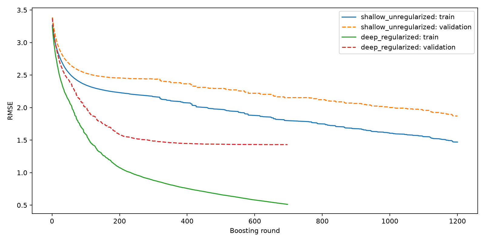
The surprising outcome is that the deeper, regularized model can outperform the shallow, unregularized model on validation data. The additional depth makes nonlinear relationships easier to express, while L1 and L2 penalties, Hessian thresholds, and row and feature sampling limit the influence of unstable corrections.
The deeper model is not automatically better. The point is that tree depth and regularization control different aspects of the learning process:
-
Depth determines which patterns the model can represent.
-
Leaf-weight penalties control the magnitude and sparsity of corrections.
-
Split and child constraints control which structures are admissible.
-
Sampling changes the observations and features available to each tree.
-
Early stopping controls how many successive corrections contribute to predictions.
A shallow model can underfit a genuinely nonlinear target. A deep model can capture that target without generalizing well if its extra capacity is unrestricted. The correct comparison is predictive performance on data that was not used to fit the model.
11. A concise decision guide when validation error diverges
When training error keeps falling but validation error starts rising, avoid increasing every penalty simultaneously. Match the intervention to the observed failure pattern.
| Failure pattern | First control to investigate | Why |
|---|---|---|
| Validation error improves, then deteriorates as rounds accumulate | Early stopping | Limits the ensemble to the useful boosting rounds. |
| Trees create deep, narrow partitions | max_depthor max_leaves |
Restricts the structural search space. |
| Small children appear to explain training noise | min_child_weight |
Requires more Hessian support for each child. |
| Individual leaf corrections appear too aggressive | reg_lambda |
Shrinks leaf weights continuously. |
| Many weak corrections appear unnecessary | reg_alpha |
Can set weak leaf weights exactly to zero. |
| Trees contain many marginal splits | gamma |
Requires sufficient loss reduction before splitting. |
| Results are sensitive to particular rows or noisy features | subsampleor colsample_bytree |
Adds randomization during tree construction. |
| Domain knowledge specifies a valid direction or forbidden interaction | Monotonic or interaction constraints | Restricts the relationships the model can represent. |
A sensible tuning order is to check the evaluation setup first, then use early stopping if divergence develops over rounds. Next, investigate tree structure and weakly supported children. Try L2 regularization and sampling when the model’s corrections or data dependence appear unstable. Consider L1 regularization and split penalties when the measured curves and tree statistics indicate that weak corrections or marginal splits are the problem.
This is a diagnostic order, not a universal ranking of hyperparameters. A model with too many tiny leaves has a different problem from one that underfits a complex target. Likewise, no regularization parameter can repair data leakage, an unsuitable loss function, or a mismatch between the training and deployment distributions.
Finally, remember that the best validation score among many tested configurations is still a model-selection result, not an unbiased estimate of production performance. Keep the test set untouched until the configuration has been selected.
Take this into your next experiment
Build a repeatable tuning loop that records training RMSE, validation RMSE, best boosting round, mean leaves per tree, and the exact configuration that produced each result. Use one-parameter sweeps to understand individual effects before testing combinations of promising settings.
Most importantly, measure both predictive performance and structure. A smaller tree is not automatically a better tree, and a larger training-validation gap is not fixed by turning every regularization control up.
Run the experiment under the pinned XGBoost 3.4.1 environment, inspect the generated CSV files and learning curves, and then apply the same controlled process to a neutral tabular dataset from your own domain. Choose the model that captures useful signal and generalizes to genuinely unseen data—not the one with the smallest trees or the lowest training error.