
LEARN · NEURAL NETWORKS FROM THE GROUND UP
A convolutional neural network does not look at an image the way a human does. It does not immediately recognize a bicycle, a building, or a handwritten digit.
Instead, it begins with small numerical patterns.
One filter might respond strongly to a vertical edge. Another might detect a horizontal stripe. A third might respond to a diagonal transition between dark and bright pixels.
As information passes through successive layers, these simple responses are combined into increasingly useful representations.
But what does that actually look like inside the network?
In this tutorial, we will go beyond architecture diagrams and inspect the computations themselves. We will implement a two-dimensional convolution using NumPy, train a small image classifier using PyTorch, and visualize both the filters it learns and the feature maps it produces.
By the end, you will understand:
-
How a convolution kernel transforms pixels into numerical responses.
-
Why convolutional layers produce multiple feature maps instead of a single image.
-
What padding, stride, activation functions, and pooling actually change.
-
How convolutional filters acquire useful patterns through training.
-
Why deeper layers see larger regions of the original image.
-
How to visualize learned filters and intermediate activations.
-
Why some learned filters resemble edge detectors found in biological vision.
We will generate our own synthetic images, so the entire experiment is reproducible and requires no external dataset downloads.
1. What a convolutional layer actually does
Imagine a grayscale image represented as a matrix of numbers.
Each pixel has an intensity, typically between 0 and 255 for an unsigned 8-bit image, or between 0 and 1 after normalization.
A simple image might contain a bright vertical bar against a dark background.
To detect that bar, we could examine every pixel individually. However, a single pixel contains almost no structural information. A bright pixel does not tell us whether it belongs to an edge, a stripe, a corner, or a large bright region.
We need to examine groups of neighboring pixels.
That is the purpose of a convolution kernel.
A kernel is a small matrix of weights
Consider this 3×3 kernel:
-1   0   1
-1   0   1
-1   0   1
The negative values examine the left side of a small image patch. The positive values examine the right side.
Suppose the patch contains dark pixels on the left and bright pixels on the right.
Multiplying each pixel by the corresponding kernel weight, then adding the results, produces a positive number.
If the brightness transition is reversed, the result becomes negative.
If the patch is completely uniform, the positive and negative contributions cancel, producing zero.
This particular kernel is therefore sensitive to horizontal changes in brightness, such as those produced by vertical edges.
The sliding-window operation
A convolutional layer applies the same kernel at many positions throughout the image.
At each position, it:
-
Extracts a patch matching the kernel’s dimensions.
-
Multiplies corresponding pixel and kernel values.
-
Adds the products.
-
Optionally adds a bias.
-
Stores the result at the corresponding output position.
The resulting matrix is called a feature map.
A feature map is not necessarily a picture of an object. It is a spatial record of how strongly a particular filter responds to the input.
Bright regions in a displayed feature map generally indicate larger numerical values under the chosen visualization scale.
One important technical detail: most deep-learning libraries, including PyTorch, implement the operation called cross-correlation, without reversing the kernel. Mathematical convolution formally reverses the kernel before applying it. In neural-network terminology, both are commonly called convolution because the filter weights are learned rather than fixed. This convention is documented in PyTorch’s current Conv2d reference.
2. Implement a 2D convolution from scratch using NumPy
Before letting a framework handle convolution, we should implement it ourselves.
Our first version will deliberately be simple:
-
A single-channel, two-dimensional image.
-
One two-dimensional kernel.
-
Configurable positive integer stride.
-
No padding.
-
No bias.
-
No activation function.
This isolates the central mathematical operation without hiding it behind framework abstractions.
The complete implementation
Save this as convolution_numpy.py.
import numpy as np


def conv2d_valid(image, kernel, stride=1):
    """Compute valid 2D cross-correlation using NumPy."""

    if image.ndim != 2 or kernel.ndim != 2:
        raise ValueError("Expected a 2D image and a 2D kernel")

    if not isinstance(stride, int) or stride < 1:
        raise ValueError("stride must be a positive integer")

    height, width = image.shape
    kh, kw = kernel.shape

    if kh > height or kw > width:
        raise ValueError("Kernel cannot be larger than the image")

    out_h = (height - kh) // stride + 1
    out_w = (width - kw) // stride + 1

    result = np.empty(
        (out_h, out_w),
        dtype=np.result_type(image, kernel, np.float32),
    )

    for i in range(out_h):
        for j in range(out_w):
            row = i * stride
            col = j * stride

            window = image[
                row:row + kh,
                col:col + kw,
            ]

            result[i, j] = np.sum(window * kernel)

    return result


image = np.array(
    [
        [0, 0, 0, 1, 1],
        [0, 0, 0, 1, 1],
        [0, 0, 0, 1, 1],
        [0, 0, 0, 1, 1],
        [0, 0, 0, 1, 1],
    ],
    dtype=np.float32,
)

vertical_edge_kernel = np.array(
    [
        [-1, 0, 1],
        [-1, 0, 1],
        [-1, 0, 1],
    ],
    dtype=np.float32,
)

response = conv2d_valid(image, vertical_edge_kernel)

print(response)

expected = np.array(
    [
        [0, 3, 3],
        [0, 3, 3],
        [0, 3, 3],
    ],
    dtype=np.float32,
)

np.testing.assert_allclose(response, expected)
The output is:
[[0. 3. 3.]
 [0. 3. 3.]
 [0. 3. 3.]]
Understanding the calculation
The input is 5×5, while the kernel is 3×3.
With stride 1 and no padding, the kernel fits into three horizontal and three vertical positions. Consequently, the result is a 3×3 feature map.
Consider the first patch, covering rows 0–2 and columns 0–2. Every pixel in that patch is zero, so its response is zero.
The next horizontal patch covers columns 1–3. It contains bright pixels in its rightmost column. Each of its three rows contributes 1 to the weighted sum, giving a result of 3.
The rightmost patch also produces 3 because its right column is bright and its left column is dark.
This tiny example captures the essential behavior of an edge detector: it responds not merely to brightness, but to a particular spatial arrangement of brightness.
What changes when the kernel changes?
Different kernels encode different preferences.
For example:
-
A vertical-edge kernel responds to changes from left to right.
-
A horizontal-edge kernel responds to changes from top to bottom.
-
A smoothing kernel averages neighboring pixels and suppresses rapid variation.
-
A sharpening kernel emphasizes differences between a pixel and its surroundings.
These are hand-designed filters.
A neural network uses the same underlying operation, but it generally learns the kernel weights from data.
That distinction is fundamental.
We do not need to specify which features are useful. We specify an architecture and a training objective, then optimize the weights so that the network can solve the task.
Our NumPy implementation also illustrates why optimized libraries matter. These nested Python loops are excellent for understanding the algorithm, but they become inefficient on large images and batches. Production frameworks use optimized CPU and accelerator kernels, while preserving the same mathematical behavior.
3. Output dimensions: why feature maps change size
A convolutional layer has several configuration parameters that determine its output.
Kernel size
A 3×3 kernel examines nine spatial positions at a time.
A 7×7 kernel examines 49 positions.
Larger kernels collect information from a larger local neighborhood, but usually require more parameters and computation when the numbers of input and output channels are unchanged.
Stride
Stride determines how far the kernel moves between adjacent output positions.
With stride 1, the kernel advances one pixel at a time.
With stride 2, it advances two pixels, reducing the spatial resolution of the output.
The kernel still performs the same weighted-sum operation; it simply evaluates fewer positions.
Padding
Without padding, convolution cannot place the kernel’s center at all boundary pixels while keeping the entire kernel inside the original image.
Padding adds extra values around the image, allowing additional positions to be evaluated.
Zero padding is common, although reflection, replication, and circular padding are also possible in supported operations.
Padding is not always visually neutral. Zero padding, for example, introduces an artificial boundary between the image and the padded region.
The output-size formula
For one spatial dimension, with dilation 1 and symmetric padding:
Output size = floor((Input size + 2 × Padding − Kernel size) / Stride) + 1
For example, with a 32-pixel-wide image, a 7-pixel-wide kernel, padding 3, and stride 1:
Output width = floor((32 + 6 − 7) / 1) + 1 = 32
The spatial size is preserved.
With zero padding and stride 2:
Output width = floor((32 − 7) / 2) + 1 = 13
The same calculation applies independently to image height.
For dilated kernels, the formula must also account for the spacing between kernel elements.
4. What happens when an image has multiple channels?
So far, our image had only one channel.
A color image usually has three: red, green, and blue.
A convolutional filter operating on a three-channel image must account for all three input channels.
For a 3×3 spatial kernel, a standard filter’s complete weight tensor therefore contains:
3 input channels × 3 rows × 3 columns = 27 weights
The layer multiplies each input-channel patch by its corresponding kernel weights and sums all the results. One bias may then be added to produce one output value.
Each complete filter produces one output feature map.
If the layer contains 16 filters, it produces 16 output channels.
For a conventional convolutional layer, the weight tensor has this shape:
(output_channels, input_channels, kernel_height, kernel_width)
This is important because a convolutional neural network does not simply keep creating grayscale versions of the original image.
It creates new collections of feature maps. Each channel represents a learned response function.
After the first layer, these channels no longer correspond directly to red, green, and blue. They represent internal features discovered through training.
That is how a network transitions from raw pixels to learned representations.
5. Build a small convolutional neural network
Now that we understand the core operation, let’s train a network and inspect what it learns.
We will use PyTorch for automatic differentiation and optimization, NumPy for synthetic data generation, and Matplotlib for visualization.
Our goal is deliberately modest: classify grayscale images containing striped patterns at different orientations.
Why stripes?
Because they make the behavior of convolutional filters relatively easy to interpret. We know the important visual property in advance: orientation.
After training, we can examine whether the network has learned filters sensitive to different directions.
Set up the environment
Use Python 3.10 or newer with a recent compatible PyTorch release.
On Linux or macOS, create a virtual environment and install the dependencies:
python -m venv .venv
source .venv/bin/activate

python -m pip install --upgrade pip
python -m pip install numpy matplotlib torch
The example runs on the CPU, so a graphics card is not required.
If you want a hardware-specific PyTorch build, particularly for CUDA or ROCm, use the commands generated by the official PyTorch installation selector.
Our synthetic dataset
Each image will be 32×32 pixels.
We will generate four categories of striped textures, corresponding to brightness variations along these directions:
-
Class 0: 0°
-
Class 1: 45°
-
Class 2: 90°
-
Class 3: 135°
The angle describes the direction in which brightness varies, which is perpendicular to the visible stripes. Thus, class 0 contains vertical stripes, while class 2 contains horizontal stripes.
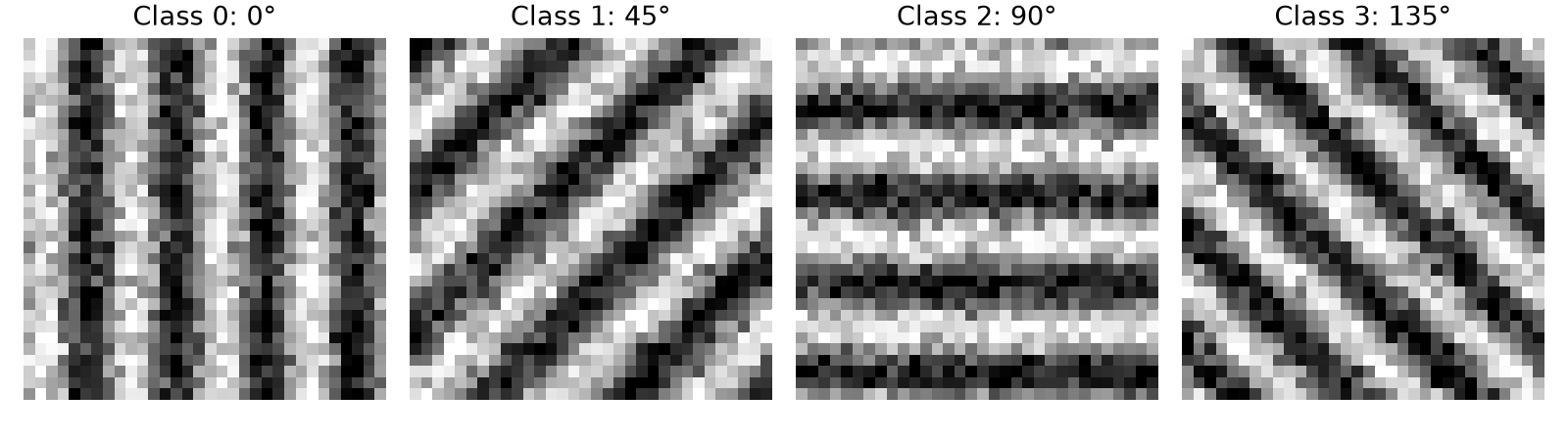
To avoid making the task completely trivial, we will vary the stripe frequency and phase and add random pixel noise.
This means the classifier must identify orientation even when the exact stripe positions and pixel values change.
We will create 1,280 training images and 320 independent validation images, each from a separate seeded random generator.
The network will have the following structure:
Input grayscale image
1 × 32 × 32
Convolution 1 — 12 filters of 7×7
12 × 32 × 32
ReLU activation → 2×2 max pooling
Intermediate feature maps
12 × 16 × 16
Convolution 2 — 16 filters of 3×3
16 × 16 × 16
ReLU activation → 2×2 max pooling
Intermediate feature maps
16 × 8 × 8
Global average pooling → 16 values
Linear classifier
4 class scores (logits)
Despite its small size, this network contains everything needed to study convolutional feature extraction: trainable filters, nonlinear activations, pooling, and classification.
6. Complete runnable training and visualization script
Save the following as cnn_visualize.py.
This script will:
-
Generate the synthetic image dataset.
-
Build and train the network.
-
Track validation accuracy.
-
Save the first-layer filters before and after training.
-
Capture intermediate feature maps for a validation image.
-
Write four PNG visualizations to the working directory.
import numpy as np
import matplotlib

matplotlib.use("Agg")

import matplotlib.pyplot as plt
import torch

from torch import nn
from torch.nn import functional as F
from torch.utils.data import DataLoader, TensorDataset


torch.manual_seed(7)
torch.set_num_threads(min(4, torch.get_num_threads()))

ORIENTATIONS = (0.0, 45.0, 90.0, 135.0)


def make_data(count, seed):
    rng = np.random.default_rng(seed)

    axis = np.arange(32, dtype=np.float32) - 15.5
    yy, xx = np.meshgrid(axis, axis, indexing="ij")

    images = np.empty(
        (count, 1, 32, 32),
        dtype=np.float32,
    )

    labels = rng.integers(
        0, 4, size=count, dtype=np.int64
    )

    for i, label in enumerate(labels):
        theta = np.deg2rad(ORIENTATIONS[label])

        distance = (
            xx * np.cos(theta)
            + yy * np.sin(theta)
        ) / 32.0

        frequency = rng.uniform(2.5, 4.5)
        phase = rng.uniform(0.0, 2.0 * np.pi)

        stripes = (
            0.5
            + 0.4
            * np.sin(
                2.0 * np.pi * frequency * distance
                + phase
            )
        )

        noise = rng.normal(
            0.0, 0.14, size=(32, 32)
        )

        images[i, 0] = np.clip(
            stripes + noise, 0.0, 1.0
        )

    return (
        torch.from_numpy(images),
        torch.from_numpy(labels),
    )


class TinyCNN(nn.Module):
    def __init__(self):
        super().__init__()

        self.conv1 = nn.Conv2d(
            1, 12, kernel_size=7, padding=3
        )

        self.conv2 = nn.Conv2d(
            12, 16, kernel_size=3, padding=1
        )

        self.pool = nn.MaxPool2d(2)
        self.classifier = nn.Linear(16, 4)

    def forward(self, x, return_features=False):
        z1 = self.conv1(x)
        a1 = F.relu(z1)
        p1 = self.pool(a1)

        z2 = self.conv2(p1)
        a2 = F.relu(z2)
        p2 = self.pool(a2)

        summary = F.adaptive_avg_pool2d(
            p2, 1
        ).flatten(1)

        logits = self.classifier(summary)

        if return_features:
            return logits, {
                "conv1": z1,
                "relu1": a1,
                "pool1": p1,
                "conv2": z2,
                "relu2": a2,
                "pool2": p2,
            }

        return logits


def evaluate(model, x, y):
    model.eval()

    with torch.inference_mode():
        logits = model(x)

        return (
            (logits.argmax(dim=1) == y)
            .float()
            .mean()
            .item()
        )


def plot_examples(x, y):
    fig, axes = plt.subplots(
        1, 4, figsize=(10, 2.8)
    )

    for label, ax in enumerate(axes):
        i = int(torch.where(y == label)[0][0])

        ax.imshow(
            x[i, 0].numpy(),
            cmap="gray",
            vmin=0,
            vmax=1,
        )

        ax.set_title(
            f"Class {label}: "
            f"{int(ORIENTATIONS[label])}°"
        )
        ax.axis("off")

    fig.tight_layout()
    fig.savefig(
        "synthetic_samples.png", dpi=160
    )
    plt.close(fig)


def plot_filters(before, after):
    scale = max(
        np.abs(before).max(),
        np.abs(after).max(),
    )

    fig, axes = plt.subplots(
        2, 12, figsize=(15, 3.5)
    )

    for row, weights in enumerate(
        (before, after)
    ):
        for channel in range(12):
            ax = axes[row, channel]

            ax.imshow(
                weights[channel, 0],
                cmap="RdBu_r",
                vmin=-scale,
                vmax=scale,
            )

            ax.set_title(
                f"F{channel}" if row == 0 else "",
                fontsize=8,
            )

            ax.axis("off")

    axes[0, 0].set_ylabel("Before")
    axes[1, 0].set_ylabel("After")

    fig.suptitle(
        "First-layer 7×7 filters: "
        "one shared color scale"
    )

    fig.tight_layout()
    fig.savefig(
        "learned_filters.png", dpi=160
    )
    plt.close(fig)


def plot_maps(
    sample, features, true_label, predicted_label
):
    names = (
        "conv1",
        "relu1",
        "pool1",
        "conv2",
        "relu2",
        "pool2",
    )

    fig, axes = plt.subplots(
        len(names), 5, figsize=(11, 14)
    )

    for row, name in enumerate(names):
        input_ax = axes[row, 0]

        input_ax.imshow(
            sample[0, 0].numpy(),
            cmap="gray",
            vmin=0,
            vmax=1,
        )

        input_ax.set_title(
            "Input", fontsize=9
        )
        input_ax.set_ylabel(
            name, fontsize=10
        )
        input_ax.set_xticks([])
        input_ax.set_yticks([])

        activations = (
            features[name][0]
            .detach()
            .numpy()
        )

        for channel in range(4):
            ax = axes[row, channel + 1]

            ax.imshow(
                activations[channel],
                cmap="magma",
                interpolation="nearest",
            )

            ax.set_title(
                f"Channel {channel}",
                fontsize=9,
            )
            ax.axis("off")

    fig.suptitle(
        f"Feature maps: true={true_label}, "
        f"predicted={predicted_label}\n"
        "Each feature map independently "
        "contrast-scaled"
    )

    fig.tight_layout()
    fig.savefig(
        "feature_maps.png", dpi=160
    )
    plt.close(fig)


def main():
    x_train, y_train = make_data(
        1280, seed=10
    )

    x_val, y_val = make_data(
        320, seed=20
    )

    plot_examples(x_val, y_val)

    loader = DataLoader(
        TensorDataset(x_train, y_train),
        batch_size=64,
        shuffle=True,
    )

    model = TinyCNN()

    before = (
        model.conv1.weight
        .detach()
        .numpy()
        .copy()
    )

    optimizer = torch.optim.Adam(
        model.parameters(), lr=0.003
    )

    criterion = nn.CrossEntropyLoss()
    accuracy_history = []

    for epoch in range(1, 11):
        model.train()
        total_loss = 0.0

        for batch_x, batch_y in loader:
            optimizer.zero_grad()

            logits = model(batch_x)
            loss = criterion(logits, batch_y)

            loss.backward()
            optimizer.step()

            total_loss += (
                loss.item() * len(batch_x)
            )

        accuracy = evaluate(
            model, x_val, y_val
        )

        accuracy_history.append(accuracy)

        print(
            f"Epoch {epoch:02d} | "
            f"train loss "
            f"{total_loss / len(x_train):.4f} | "
            f"validation accuracy "
            f"{accuracy:.1%}"
        )

    after = (
        model.conv1.weight
        .detach()
        .numpy()
        .copy()
    )

    plot_filters(before, after)

    fig, ax = plt.subplots(
        figsize=(5.5, 3.5)
    )

    ax.plot(
        range(1, len(accuracy_history) + 1),
        accuracy_history,
        marker="o",
    )

    ax.set(
        xlabel="Epoch",
        ylabel="Validation accuracy",
        ylim=(0, 1.05),
    )

    ax.grid(alpha=0.3)
    fig.tight_layout()

    fig.savefig(
        "training_curve.png", dpi=160
    )
    plt.close(fig)

    index = int(
        torch.where(y_val == 2)[0][0]
    )

    sample = x_val[index:index + 1]

    model.eval()

    with torch.inference_mode():
        logits, feature_maps = model(
            sample,
            return_features=True,
        )

    predicted = int(
        logits.argmax(dim=1).item()
    )

    plot_maps(
        sample,
        feature_maps,
        int(y_val[index]),
        predicted,
    )

    for name, tensor in feature_maps.items():
        print(
            f"{name:>5}: "
            f"{tuple(tensor.shape)}"
        )

    print(
        "Saved: synthetic_samples.png, "
        "learned_filters.png, "
        "training_curve.png, "
        "feature_maps.png"
    )


if __name__ == "__main__":
    main()
Run the script:
python cnn_visualize.py
The training loop uses standard PyTorch operations: forward propagation, cross-entropy loss, automatic differentiation, and Adam optimization.
Each optimizer step updates the filters according to how their current responses affect the classification error. The current PyTorch training documentation describes this workflow in more detail.
On a CPU test run, the model reached 100% validation accuracy by the second epoch and maintained it over the remaining epochs. Exact results may vary across versions, hardware, and random-number implementations.
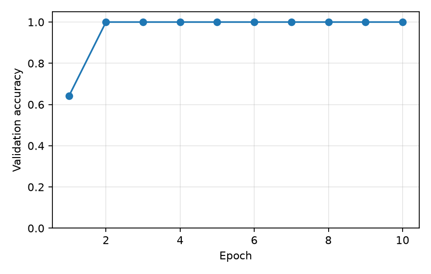
That high accuracy is unsurprising for a small synthetic dataset with well-separated orientation classes. It should not be interpreted as evidence that the model understands arbitrary natural images.
7. Visualizing what the first layer learned
The first visualization to inspect is the filter comparison.
The script produces these files:
synthetic_samples.png
learned_filters.png
training_curve.png
feature_maps.png
Open learned_filters.png.
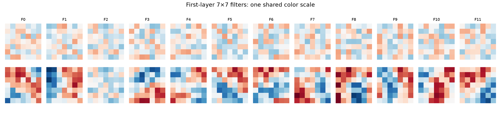
The first row contains the 12 initial filters. The second row contains the same filters after training.
Before training, the weights appear approximately random. There is no obvious spatial arrangement that consistently corresponds to an orientation.
After training, some filters develop recognizable structure: alternating positive and negative regions, directional bands, and other patterns that are useful for distinguishing the synthetic textures.
This is learning made visible.
Why negative weights are useful
Consider a filter with positive weights on one side and negative weights on the other.
When an image patch matches that arrangement, the weighted sum becomes strongly positive.
When the brightness transition runs in the opposite direction, the response may become negative.
The network can exploit this sign difference, although a subsequent ReLU will suppress negative activations.
A learned kernel is therefore more than a brightness detector. It can encode spatial contrast, orientation, and local frequency preferences.
Why comparing before and after matters
A filter visualization shown only after training can be misleading.
A random initialization may already contain small accidental patterns that look vaguely like edges.
Comparing the same filters before and after optimization lets us distinguish initial randomness from systematic changes acquired during training.
Our plotting code also uses one shared color scale for both rows. This prevents changes in automatic color normalization from masquerading as changes in the weights.
Why we visualize only the first layer’s weights
The first convolution receives one grayscale input channel, so each filter is a single 7×7 matrix that can be displayed as an image.
The second convolution receives 12 channels.
Each second-layer filter therefore consists of 12 separate 3×3 matrices, not one straightforward grayscale image.
You can visualize those channel slices individually, but interpreting the entire second-layer filter requires considering how it combines multiple earlier feature maps.
This is one reason first-layer filters are especially popular in neural-network visualization.
8. What feature maps reveal, layer by layer
The most informative file is feature_maps.png.
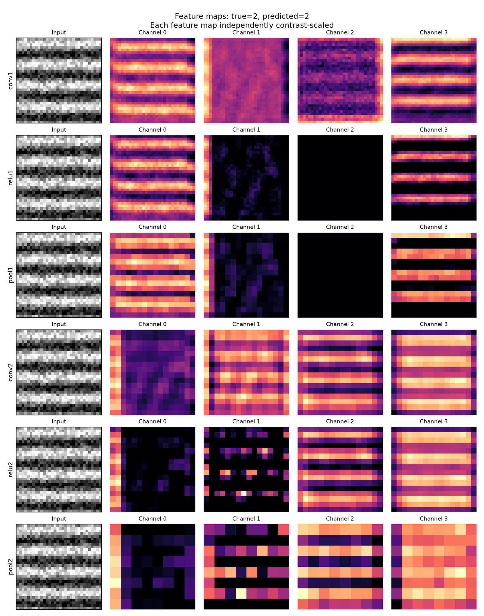
It shows one held-out validation image alongside four feature channels from each of six processing stages.
We repeat the input image in the first column for reference.
The selected image belongs to class 2, representing a texture with horizontal stripes.
The rows illustrate how the network transforms those stripes into numerical representations.
Layer 1: Raw convolution responses
The first convolution produces 12 feature maps, each with a spatial size of 32×32.
Each filter sees a local 7×7 region and computes a weighted sum.
Suppose a filter has become sensitive to horizontal banding.
Its feature map may contain strong responses at locations where the input exhibits that pattern. A filter with a different orientation preference may produce weaker responses.
Importantly, these are pre-activation values.
They can be positive, negative, or zero.
At this point, the convolution itself is a linear operation plus a bias.
Layer 2: ReLU activation
ReLU stands for Rectified Linear Unit.
It applies the following transformation independently to every activation:
ReLU(x) = max(0, x)
Positive values remain unchanged, while negative values become zero.
For example:
Before ReLU:
-2   1  -3
 4  -1   5

After ReLU:
 0   1   0
 4   0   5
Why introduce this transformation?
Without nonlinear activation functions, a sequence of ordinary convolutional and fully connected linear layers would still represent a linear transformation of the input, assuming no other nonlinear operations intervene.
ReLU allows the network to construct nonlinear decision functions.
In our visualization, you should notice that some regions become exactly zero after ReLU.
A feature map may even be entirely zero for the selected input if all its pre-activation values are nonpositive.
That does not necessarily mean its filter is useless. It may respond strongly to different images.
Layer 3: First max-pooling operation
Next comes 2×2 max pooling with stride 2.
Each nonoverlapping 2×2 region is replaced by its maximum value.
For example:
Input patch:
1  3
2  5

Pooled result:
5
Pooling reduces each spatial dimension from 32 to 16.
The output therefore contains 12 feature maps of size 16×16.
Pooling makes the representation smaller and preserves strong local activations. For small shifts within a pooling window, the maximum may remain unchanged, creating a degree of local shift tolerance.
But max pooling is not perfectly translation-invariant.
Moving a feature across pooling-window boundaries may change the output substantially.
Pooling also discards information. The three nonmaximum values in each region are not preserved.
That tradeoff is useful when a task depends more on the presence of local features than on their exact pixel coordinates.
Layer 4: Second convolution
Now the network has 12 input feature channels rather than one raw image channel.
The second convolution uses 16 filters, each with dimensions 12×3×3.
It produces 16 output maps of size 16×16.
Each output combines information from every input channel in the standard, ungrouped convolution used here.
Instead of detecting an edge directly from pixel intensities, a second-layer filter can learn relationships among earlier responses.
For instance, it might respond to a combination of two oriented patterns or to a particular arrangement of contrast features.
For this stripe-classification task, second-layer features can help distinguish the frequency and orientation patterns represented by earlier filters.
Do not expect every channel to resemble a clean, human-recognizable shape. Internal representations are optimized for the training objective, not for producing attractive visualizations.
Layer 5: Second ReLU
The second activation again removes negative values.
This allows the network to create more selective nonlinear responses from the combinations produced by the second convolution.
Some channels may activate strongly for the selected orientation. Others may be mostly inactive.
A bright feature map is not automatically more important than a dark one.
The final classifier determines how the different channels contribute to each class score.
Layer 6: Second max pooling
The final max-pooling operation reduces the spatial dimensions from 16×16 to 8×8.
We now have 16 feature maps, each containing 64 spatial positions.
The network then applies global average pooling.
Instead of flattening all 1,024 remaining values, it calculates one average value per channel.
This produces a 16-element feature vector.
A final linear layer converts those 16 values into four class scores, called logits. The class with the highest logit is the predicted class.
Because cross-entropy loss accepts logits directly, our training implementation does not need to apply softmax explicitly before computing the loss.
The complete shape transformation
| Stage | Output shape for one image |
|---|---|
| Input | 1 × 32 × 32 |
| First convolution | 12 × 32 × 32 |
| First ReLU | 12 × 32 × 32 |
| First max pooling | 12 × 16 × 16 |
| Second convolution | 16 × 16 × 16 |
| Second ReLU | 16 × 16 × 16 |
| Second max pooling | 16 × 8 × 8 |
| Global average pooling | 16 values |
| Linear classifier | 4 logits |
The important observation is that spatial resolution gradually decreases while the number of feature channels initially increases.
The network exchanges some spatial detail for increasingly processed representations.
9. Receptive fields: how deeper layers see more
A subtle property of convolutional networks is that deeper neurons have larger receptive fields.
The receptive field of a neuron is the region of the original input that can influence that neuron’s activation.
In the first convolution, a neuron depends on a 7×7 patch of the original image.
After the first 2×2 pooling operation, each pooled activation can depend on an 8×8 region.
The second convolution combines neighboring pooled activations.
Because its kernel is 3×3 and neighboring pooled positions are separated by two input pixels, an output activation of the second convolution has a theoretical receptive field of 12×12 pixels.
After the second pooling operation, the theoretical receptive field becomes 14×14.
These values describe the maximum nominal support in the original image; boundary padding means edge positions may include padded values.
The progression is:
Conv 1
7×7
Pool 1
8×8
Conv 2
12×12
Pool 2
14×14
Conceptual receptive-field sizes within the original 32×32 input. Boxes are centered for illustration.Notice that the receptive field increases even though the feature maps become smaller.
This is one reason deep convolutional networks can represent larger structures: later units can combine information from increasingly extensive regions of the input.
However, a theoretical receptive field is not the same as an effective receptive field.
In practice, different input positions can contribute with different strengths. Some locations inside the theoretical region may have very little influence on a particular activation.
Global average pooling aggregates information from all spatial positions in the final feature maps, so the final classifier can depend on evidence distributed throughout the input image.
10. Cherry on the cake: why learned filters often look like Gabor filters
One of the most interesting observations in computer vision is that early convolutional filters can develop patterns resembling Gabor filters.
A Gabor filter consists of an oscillating pattern, often a sine or cosine wave, multiplied by a localized Gaussian envelope.
Visually, it resembles alternating bright and dark bands that fade away from the center.
Gabor filters have several useful properties:
-
They respond to particular orientations.
-
They respond to particular spatial frequencies.
-
They emphasize localized texture and edge information.
-
Collections of filters at different orientations and frequencies can describe complex textures.
These properties make them useful in classical image processing.
They are also related to orientation-selective responses observed in simple cells of the primary visual cortex. Current scikit-image documentation illustrates this relationship through Gabor filter banks for texture classification.
The surprising part
A convolutional neural network does not need to be explicitly instructed to detect edges or learn Gabor-like patterns.
Given an appropriate visual dataset and optimization objective, gradient-based training can discover that orientation-sensitive filters are useful.
Why?
Because many visual distinctions depend on local changes in intensity.
A filter that recognizes an oriented contrast pattern can become useful to many downstream computations.
During training, filters that improve the network’s predictions receive weight updates that reinforce their usefulness.
This can lead to oriented, alternating positive-negative patterns emerging from initially random weights.
Does every convolutional network discover Gabor filters?
No.
The appearance of learned filters depends on:
-
The images used for training.
-
The task and loss function.
-
The filter dimensions.
-
The architecture and initialization.
-
The optimization process.
Some filters resemble clean directional edges. Others resemble blobs, gradients, or more irregular patterns.
In our synthetic experiment, several filters develop visible orientation structure, but they are not guaranteed to become perfect mathematical Gabor functions.
This is an important distinction between observing a resemblance and proving that the network has learned a specific predefined filter family.
The deeper lesson is more interesting than any single filter shape: a useful representation can emerge from optimizing a task, rather than from explicitly programming the representation itself.
11. Three visualization mistakes to avoid
Once you start visualizing neural networks, it becomes tempting to interpret every colorful heatmap as a meaningful discovery.
That is risky.
Mistake 1: Confusing a filter with a feature map
A filter is a set of learned parameters.
A feature map is the result of applying a filter, or a sequence of operations, to a particular input.
The filter remains fixed during inference. Its feature map changes when the input changes.
For example, the same vertical-edge detector can produce strong responses on one image and almost no response on another.
When interpreting a visualization, always ask whether you are looking at the model’s weights or at an activation produced for an image.
Mistake 2: Ignoring color normalization
Matplotlib typically scales each displayed image according to its own minimum and maximum values unless you specify otherwise.
This means two feature maps with very different numerical magnitudes can appear equally bright.
Our feature-map visualization intentionally uses independent contrast scaling so that spatial patterns are visible in each panel.
It is suitable for examining where a channel responds, but not for quantitatively comparing response strength across different channels or layers.
For quantitative comparisons, use a consistent scale, inspect numerical summaries, or compare the original activation values.
Mistake 3: Assuming a bright region explains a prediction
A feature map shows where an intermediate channel responds.
It does not, by itself, establish that the region caused the final prediction.
Some channels can contribute positively to one class and negatively to another through later learned weights.
A large activation may ultimately have little effect on the selected class.
To investigate prediction-specific influence, you need additional analysis such as gradient-based attribution, perturbation experiments, or other carefully chosen interpretability techniques.
Activation visualization is an excellent starting point, but it is not a complete explanation of model behavior.
12. Experiments to deepen your understanding
The strongest way to understand convolution is to modify the working code and observe the consequences.
Here are several experiments worth trying.
Experiment A: Increase the stride
Change the first convolution to use stride 2.
Predict the first feature-map dimensions before running the code.
Then consider why the feature maps become smaller and what spatial information is no longer sampled.
You will also need to account for the changed feature-map sizes when interpreting the later layers.
Experiment B: Reduce the number of filters
Change the first layer from 12 filters to four.
Update the second convolution’s input-channel count accordingly.
Retrain the network and compare the validation accuracy and learned filters.
Does the model still distinguish the four orientations reliably?
A smaller filter bank may be sufficient for this simple task, but reducing channels also reduces representational capacity.
Experiment C: Make the dataset harder
Increase the amount of image noise, vary stripe frequencies over a wider range, or introduce small rotations away from the four exact orientations.
This makes the training distribution more varied and the classes potentially less separable.
Observe how the learned filters and validation accuracy change.
Experiment D: Test spatial shifts
Generate an image with the same orientation but a different phase, effectively shifting the stripe pattern.
Observe how feature maps move or change.
This illustrates the relationship between convolution and translation equivariance.
A stride-1 convolution without boundary effects is translation-equivariant: shifting the input shifts the response correspondingly.
But finite-image padding, strided operations, pooling, and global aggregation can alter this behavior.
Translation equivariance and translation invariance are different properties, and neither should be assumed for an entire network without examining its operations.
Experiment E: Compare learned filters with fixed filters
Create several manually designed oriented edge detectors and apply them to the same synthetic image.
Compare their responses against the learned filters.
This experiment helps separate two questions:
-
Can a filter detect a particular pattern?
-
Is that filter useful for the objective being optimized?
A carefully hand-designed filter might be visually easy to interpret but less useful for a specific training objective than a less recognizable learned filter.
13. What this teaches us about convolutional networks
It is easy to describe a convolutional neural network as a system that recognizes increasingly complex visual features.
That description is useful, but incomplete.
The more precise story is that the network repeatedly transforms arrays of numbers using trainable local filters, nonlinear functions, spatial aggregation, and learned combinations of channels.
In our experiment, this process starts with grayscale pixels and ends with four orientation scores.
Along the way:
-
The first convolution computes local weighted sums.
-
ReLU introduces nonlinear behavior and suppresses negative activations.
-
Max pooling reduces spatial resolution while preserving local maxima.
-
The second convolution combines responses from earlier channels.
-
Global average pooling summarizes each final channel.
-
The classifier converts the resulting feature vector into class scores.
-
Backpropagation updates the filters according to their contribution to the loss.
Nothing in the architecture explicitly states that horizontal, vertical, or diagonal patterns must be detected.
Those preferences develop because they are useful for classifying our data.
That is the essential insight behind learned visual representations.
A network’s internal features are not selected by a human naming objects and edges. They are shaped by the interaction between architecture, data, and optimization.
14. Further reading
If you want to continue from this experiment into more advanced convolutional networks, these resources provide useful next steps.
-
PyTorch Conv2d documentation — detailed specifications for convolution parameters, output shapes, and weight tensors.
-
PyTorch neural-network training tutorial — how loss functions, automatic differentiation, and optimizers work together.
-
scikit-image Gabor filter examples — practical examples of orientation-sensitive filtering.
-
Feature Visualization, Distill — foundational research explaining how neural-network activations can be explored through optimized inputs.
Your next step: make the network show you what it learned
Run the NumPy implementation first. Verify that you can explain every number in its output.
Then train the PyTorch model and open all four generated visualizations.
Start with the learned filters. Identify any directional patterns. Move to the feature maps and compare the raw convolution responses with their post-ReLU and post-pooling versions.
Finally, make one architectural change and repeat the experiment.
Your challenge: train the same network on six or eight stripe orientations instead of four. Increase the output classes accordingly, inspect the new learned filters, and compare the results with the original model.
You will move from simply recognizing a convolutional layer in a diagram to understanding what its filters compute, what its activations represent, and how training changes the information flowing through the network.
That is the point where convolutional networks stop feeling like black boxes and start becoming systems you can investigate, test, and reason about.